lylyhs / predicting_respiratory_rate

Predicting respiratory rate using PPG and ECG data available on smart devices

Predicting Respiratory rate using data available on a smart watch

April 2019

by Joe Ganser

ABSTRACT

This research was the product of a data driven healthcare hackathon I participated sponsored by Accenture and the School of AI. I was the team leader, and our team came in first place for the NY division. Here we use blood oxygen and electrocardiogram data to predict the rate at which people breath. It turns out, this data can be extracted from a smart watch. Using this data, we could predict a persons respiratory rate with 90% accuracy.

CONTENTS

• I. Introducing the problem
  • I.A Background information & Context
  • I.B The goals of this analysis
• ** II. Data Structure & Feature Engineering**
  • II.A How the data was originally harvested
  • II.B The original data's structure: ECG, PPG & pulminory
  • II.C Visualizing the fundamental data
  • II.D Engineering the features
• ** III. Putting the big data on Amazon Web Service**
• IV. Modelling
  • IV.A Assumptions that had to be made
  • IV.B Model deployment
  • IV.C Best Results
  • IV.D Validating a well fit model
  • IV.E Feature importance
• V. Conclusions
  • V.A Insights on usage
  • V.B Prospects on further deployment
• VI. Links to Coded Notebooks
• VII. References

Our official presentation title

I. Introducing the problem

Background information & Context

Electrocardiogram (ECG) data and photoplethysmogram (PPG) data are extremely useful in healthcare. They are used to assist in diagnostic methods for a wide array of diseases. ECG measures cardiac properties and PPG data measures blood oxygen levels using optical instruments. (1,2)

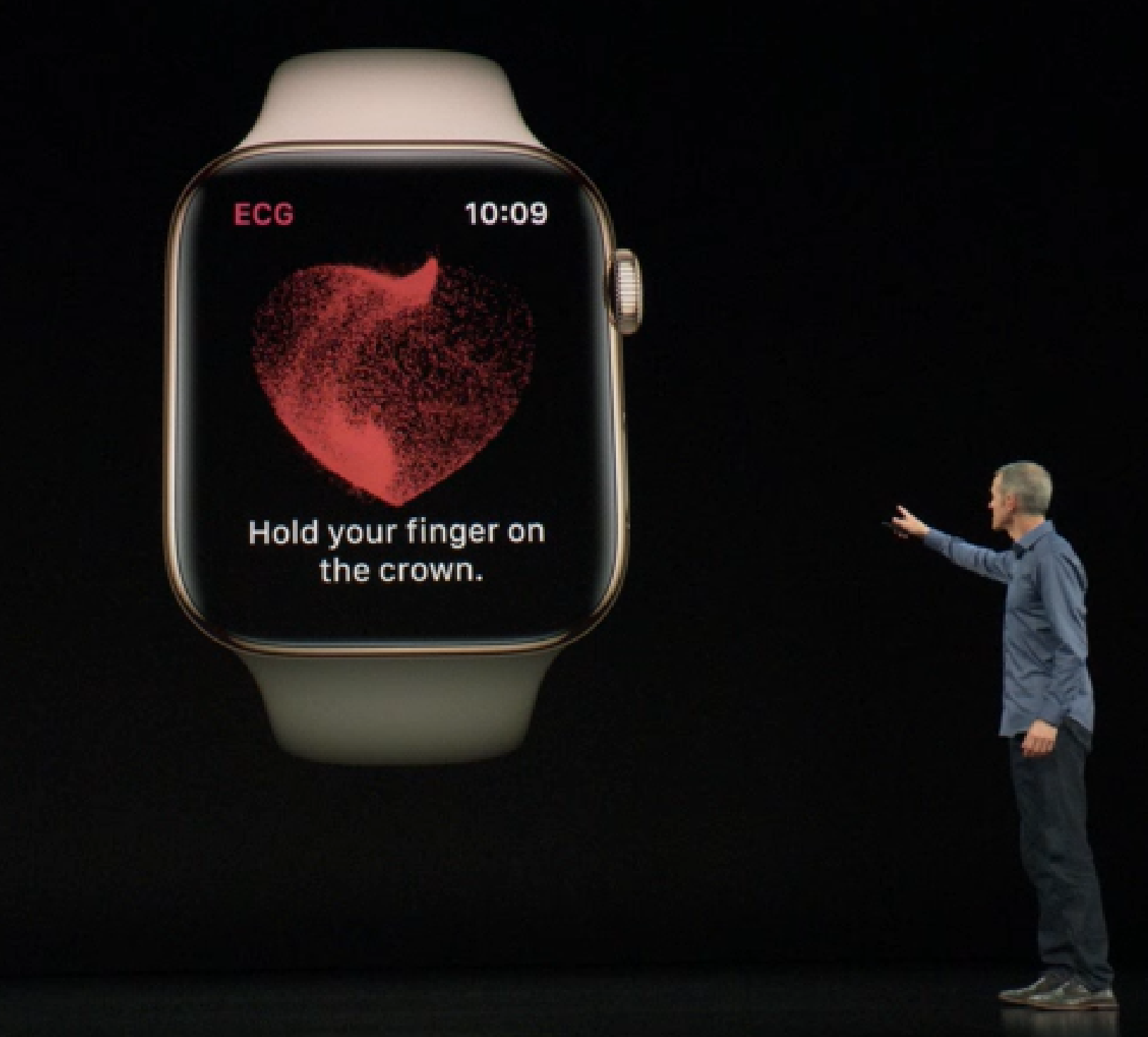
Both ECG and PPG data can be extracted from a smart watch at the same level of accuracy and precisions of machines found in hospitals. ECG and PPG can be combined to predict breathing rate, and using the combination of all this data (3,4,5).

The data used for this analysis was not actually collected from a smart watch, but smart watches have the capability to collect the same data. The data used in this analysis was from 53 patients in intensive care, where their ECG, PPG and breathing rates were measured. (4,5,6)

Goals of the analysis

The goal was to use supervised machine learning techniques to predict a persons breathing rate using real time, continuous PPG and ECG data.

In conjunction, it was also our goal to investigate the feasibility of using this type of data for enhancing diagnostic processes in healthcare. We ended by speculating on the market evolution of technology that integrates these methods.

II. Data Structure & Feature Engineering

How the data was originally harvested

The data used for this analysis was time series recorded from 53 ICU patients, in age ranges between 19-84. Both male and female patients were present. They were recorded using hospital based ECG and PPG devices, and a breathing apparatus. Continuous measurements for each patient were made across apporximately 8 minutes (6).

The original data's structure: ECG, PPG & pulminory

The data was aggregated from two fundamental sources - one which was collected at 1Hz and the other at 125Hz. These were then joined in a left outer manor. Some of the key features were;

• Respiratory rate (the supervised learning target)
• Pulse
• Blood oxygen level
• Pleth (pulmonary data)
• V (voltage)
• AVR
• II

The 1Hz data looked like this;

Time (s)	HR	PULSE	SpO2
0	93	92	96
1	92	92	96
2	92	92	96
3	92	93	96
4	92	93	96

The 125Hz data looked like this;

Time (s)	RESP	PLETH	II	V	AVR
0.0	0.25806	0.59531	-0.058594	0.721569	0.859379
0.008	0.26393	0.59042	-0.029297	0.69608	0.69531
0.016	0.269790	0.58358	0.179690	0.7	0.45508
0.024	0.27566	0.57771	0.84375	0.32941	0.041016
0.032	0.2825	0.57283	1.3184	0.078431	-0.099609

After combining with left outer join, we got;

Time (s)	RESP	PLETH	V	AVR	II	HR	PULSE	SpO2
0.0	0.25806	0.59531	0.721569	0.859379	-0.0585944	93	92	96
0.008	0.26393	0.59042	0.69608	0.69531	-0.029297	93	92	96
0.016	0.269790	0.58358	0.7	0.45508	0.17969	93	92	96
0.024	0.27566	0.57771	0.32941	0.041016	0.84375	93	92	96
0.032	0.2825	0.57283	0.078431	-0.099609	1.3184	93	92	96

For each person in the study, this amounted to about 60,000 rows. When all 53 people were combined, we were left with approximately 2.7 million rows (about 1.2Gb of data.)

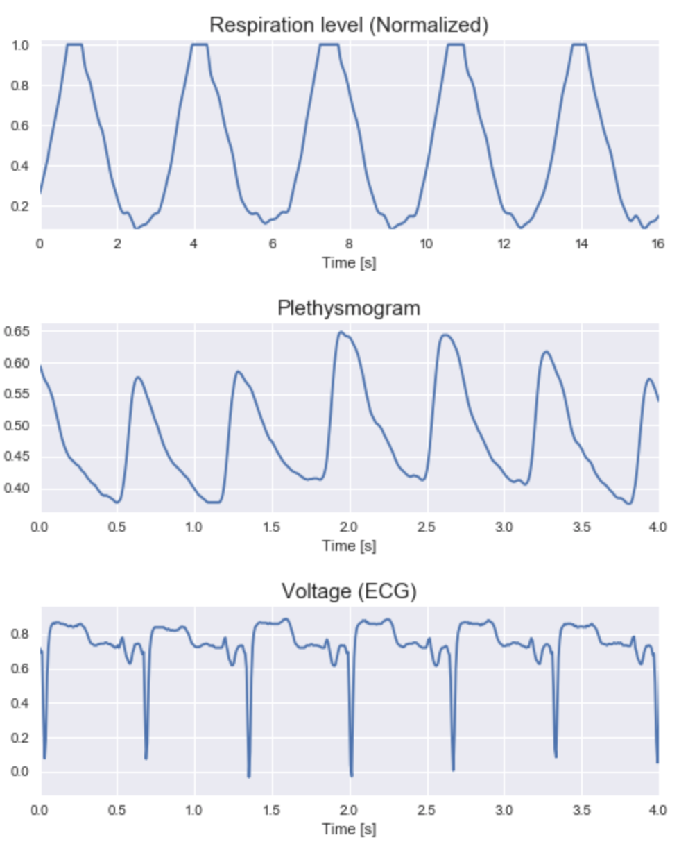
Visualizing the fundamental data

The data was fundamentally time series based. Here are a few snapshots of some of the key features;

Feature engineering

Considering the aggregation of the data from 125Hz, the values of the metrics varied quite a bit in each second. Thus, summary statistics of the 125 values collected each second could be engineered into features. Specifically, these features were;

• Max value
• Min value
• Mean value
• Kurtosis value
• Skew value

(Over the distribution of the 125 measurements made each second). To create these features, a function was created.

from scipy.stats import kurtosis,skew

def make_features(frame):
    frame.fillna(numerics.mean(),inplace=True) 
    Hz_125_cols = [' RESP', ' PLETH', ' V', ' AVR', ' II']
    Min = frame[Hz_125_cols+['sec']].groupby('sec').min()
    Min.columns = [i+'_Min' for i in Min.columns]
    Max = frame[Hz_125_cols+['sec']].groupby('sec').max()
    Max.columns = [i+'_Max' for i in Max.columns]
    Mean = frame[Hz_125_cols+['sec']].groupby('sec').mean()
    Mean.columns = Mean.columns = [i+'_Mean' for i in Mean.columns]
    Kurt = frame[Hz_125_cols+['sec']].groupby('sec').agg(lambda x: kurtosis(x))
    Kurt.columns = [i+'_Kurt' for i in Kurt.columns]
    Skw = frame[Hz_125_cols+['sec']].groupby('sec').agg(lambda x: skew(x))
    Skw.columns = [i+'_Skw' for i in Skw.columns]
    summary_frames = [Min,Max,Mean,Kurt,Skw]
    one_sec_summary = pd.concat(summary_frames,axis=1).reset_index()
    frame = frame.merge(one_sec_summary,on='sec',how='outer')
    return frame

Time (s)	RESP	PLETH	V	AVR	II	HR	PULSE	SpO2	RESP_Min	PLETH_Min	V_Min	AVR_Min	II_Min	RESP_Max	PLETH_Max	V_Max	AVR_Max	II_Max	RESP_Mean	PLETH_Mean	V_Mean	AVR_Mean	II_Mean	RESP_Kurt	PLETH_Kurt	V_Kurt	AVR_Kurt	II_Kurt	RESP_Skw	PLETH_Skw	V_Skw	AVR_Skw	II_Skw
0.0	0.25806	0.59531	0.72157	0.85938	-0.05859	93	92	96	0.25806	0.37732	0.07451	-0.09961	-0.21484	1.0	0.59531	0.87059	1.0254	1.3438	0.70822	0.46446	0.75551	0.81947	-0.02431	-1.40052	-1.08775	10.3465	13.15985	13.94906	-0.24258	0.48232	-3.05758	-3.3357	3.5823
0.008	0.26393	0.59042	0.69608	0.69531	-0.0293	93	92	96	0.25806	0.37732	0.07451	-0.09961	-0.21484	1.0	0.59531	0.87059	1.0254	1.3438	0.70822	0.46446	0.75551	0.81947	-0.02431	-1.40052	-1.08775	10.3465	13.15985	13.94906	-0.24258	0.48232	-3.05758	-3.3357	3.5823
0.016	0.26979	0.58358	0.7	0.45508	0.17969	93	92	96	0.25806	0.37732	0.07451	-0.09961	-0.21484	1.0	0.59531	0.87059	1.0254	1.3438	0.70822	0.46446	0.75551	0.81947	-0.02431	-1.40052	-1.08775	10.3465	13.15985	13.94906	-0.24258	0.48232	-3.05758	-3.3357	3.5823
0.024	0.27566	0.57771	0.32941	0.04102	0.84375	93	92	96	0.25806	0.37732	0.07451	-0.09961	-0.21484	1.0	0.59531	0.87059	1.0254	1.3438	0.70822	0.46446	0.75551	0.81947	-0.02431	-1.40052	-1.08775	10.3465	13.15985	13.94906	-0.24258	0.48232	-3.05758	-3.3357	3.5823
0.032	0.2825	0.57283	0.07843	-0.09961	1.3184	93	92	96	0.25806	0.37732	0.07451	-0.09961	-0.21484	1.0	0.59531	0.87059	1.0254	1.3438	0.70822	0.46446	0.75551	0.81947	-0.02431	-1.40052	-1.08775	10.3465	13.15985	13.94906	-0.24258	0.48232	-3.05758	-3.3357	3.5823

III. Putting the big data on Amazon Web Service

During the hackathon, Accenture provided us with a $125 gift certificate to create and Amazon Web Service EC2 instance.

This enabled us to use a p3.2x large instance, putting 1.2Gb into the system. Despite our enhanced processing capability, it was still challenging and time consuming to run all the models. It took approximately 6-10 minutes to run the full models on AWS.

IV. Modelling

Multiple attempts using regression techniques were made to model the data. Using resp as our target, our goal was to optimize performance on the metrics of;

• R2 score
• Mean squared error
• Model evaluation time (seconds)

Assumptions that had to be made

To make a regression analysis on time series data, we had to assume the time series is itself stationary. This means that the value of the feature we're analyzing has an average and variance that is constant in time.

Stated mathematically, the assumptions were;

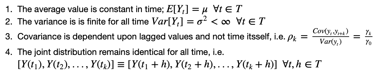
Are these assumptions valid or realistic? Yes definitiely so. Why? Because the people who were being studied in the original analysis for which the data is being collected were laying down in bed throughout the study. Thus, the there was no stimulus to change in the time series, and it can be assumed to have a constant trend.

Model Development

A function was created to put the data through a pipeline for which it was fitted and scored on several different types of models. The models that were compared were

• Ordinary Least Squares
• Lasso Regression
• Elastic Net Regression
• Ridge regression
• Bayesian Ridge
• K-neighbors regression
• Random Forest Regression

The function that produced this system was this;

import time
import numpy as np
from sklearn.metrics import r2_score,mean_squared_error,mean_absolute_error
from sklearn.linear_model import Lasso,Ridge,ElasticNet, BayesianRidge, LinearRegression
from sklearn import neighbors
from sklearn.ensemble import RandomForestRegressor
from sklearn.model_selection import train_test_split

models = {'OLS':LinearRegression(),'ElasticNet':ElasticNet(),
          'BayesianRidge':BayesianRidge(),'Lasso':Lasso(),
         'Ridge':Ridge(),'KNN':neighbors.KNeighborsRegressor(),
         'rff':RandomForestRegressor()}

def model_performance(X,y):
    times =[]
    keys = []
    mean_squared_errors = []
    mean_abs_error = []
    R2_scores = []
    X_train, X_test, y_train, y_test = train_test_split(X, y, test_size=0.3, random_state=10)

    for k,v in models.items():
        model = v
        t0=time.time()
        model.fit(X_train, y_train)
        train_time = time.time()-t0
        t1 = time.time()
        pred = model.predict(X_test)
        predict_time = time.time()-t1
        pred = pd.Series(pred)
        Time_total = train_time+predict_time
        times.append(Time_total)
        R2_scores.append(r2_score(y_test,pred))
        mean_squared_errors.append(mean_squared_error(y_test,pred))
        mean_abs_error.append(mean_absolute_error(y_test,pred))
        keys.append(k)
    table = pd.DataFrame({'model':keys, 'RMSE':mean_squared_errors,'MAE':mean_abs_error,'R2 score':R2_scores,'time':times})
    table['RMSE'] = table['RMSE'].apply(lambda x: np.sqrt(x))
    return table

model_performance(X,y)

Best Results

After running this function, we got a table of performance metrics for each model. Note this is when we run on one only one person's data. If we ran on everyone in the study, the metrics were approximately the same.

model	R2 score	time(s)	RMSE
Random Forest	0.90017	2.85901	0.11014
KNN	0.82439	4.02399	0.12569
BayesianRidge	0.53836	0.076529	0.203805
Ridge	0.53835	0.02263	0.20380
OLS	0.53835	0.36989	0.20380
ElasticNet	-1.24037e-05	0.02514	0.29996
Lasso	-1.24037e-05	0.02388	0.29996

Clearly, it was the random forest regressor that achieved the best results.

Validating a well fit model

Aside from simply metrics of performance, it's also good to look at how well the model has been fit. Here we see distribution of errors on the train set and the test set;

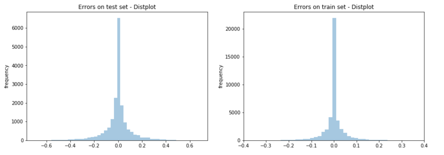
The frequency count may be slightly different in scale, but this is ok because its size difference is proprotional to the size differences in the train set and the test set.

Feature importance

One of the beauties of the random forest package, is it allows us to create an output describing the magnitude of feature importances.

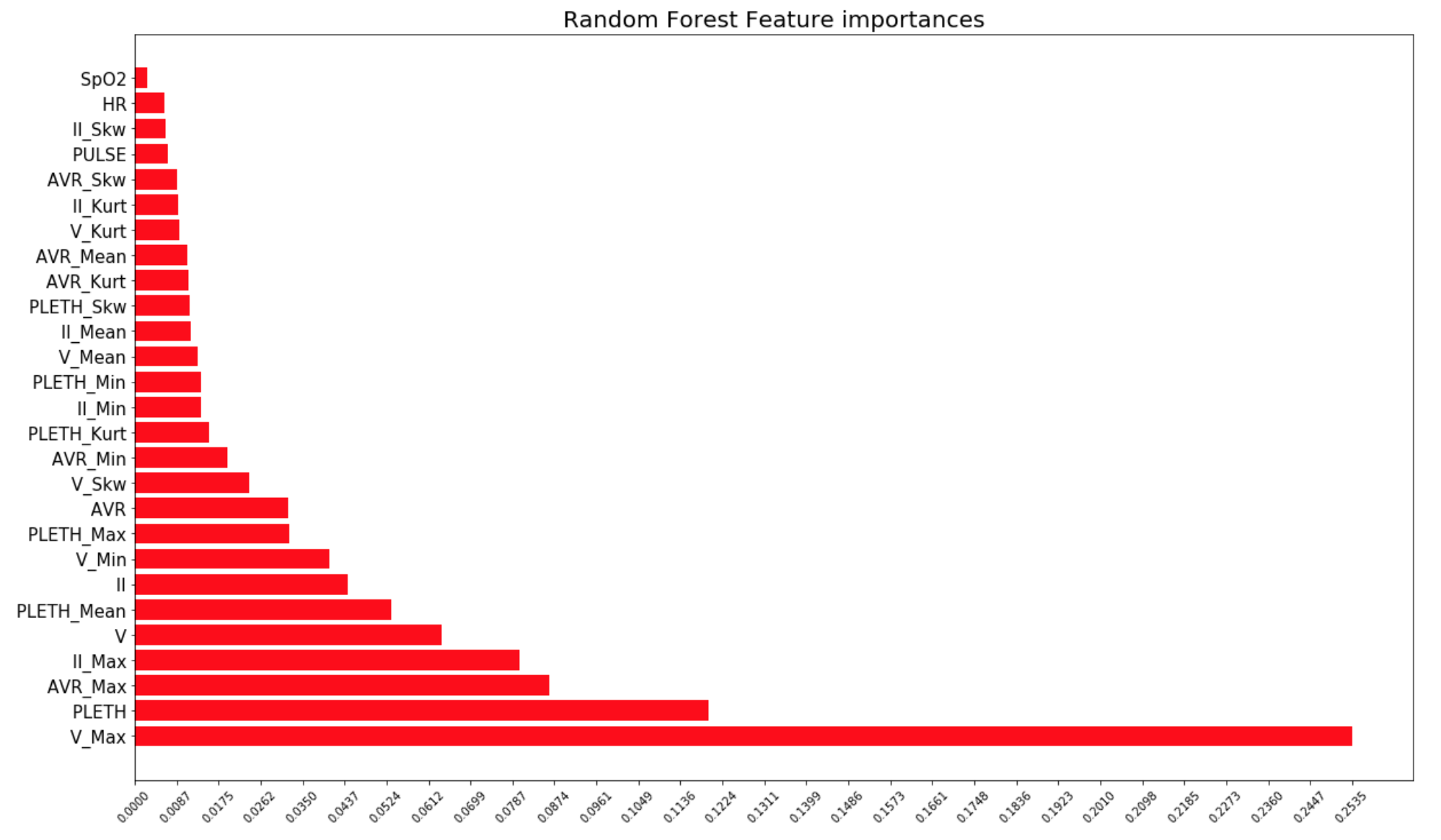
It was also noticed that if we eliminated the plethysmogram data, we could still predict breathing rate with upto about 80% accuracy.

V. Conclusions

We can draw a few conclusions.

• Using a persons plethysmogram and electrocardiogram data we can predict their respiratory rate with 90% accuracy.
• If we train on multiple people's data, we predict anyone's respiratory rate with very good data.

Insights on usage

Being able to predict user's breathing rate with home based wearable technology opens up a lot of opportunities for healthcare. This can allow us to do things such as;

• Have doctors monitor our health at home
• Enhance and assist with continuous health monitoring
• Prevent major health crises before they occur.

Prospects on further usage

Perhaps these algorithms and data collection techniques can be put into smart watch/phone apps. Software could be created that allows for automation of doctor patient interaction, notifying healthcare professionals in real time when a serious issue arises.

Smart watches might save lives one day!

VI. Links to coded notebooks

• Downloading and aggregating the data
• Modelling the data
• Random forest performance

VII. References

1. Electrocardiogram (ECG) https://en.wikipedia.org/wiki/Electrocardiography
2. Photoplethysmogram (PPG) https://en.wikipedia.org/wiki/Photoplethysmogram#Photoplethysmograph
3. Probabilistic Estimation of Respiratory Rate from Wearable Sensors, Pimentel, Charlton, Clifton, Institute of Biomedical Engineering, Oxford University http://www.robots.ox.ac.uk/~davidc/pubs/springer2015.pdf
4. PPG data can be extracted using smart watches: https://www.ncbi.nlm.nih.gov/pubmed/26737690
5. ECG data cen be extracted using smart watches: https://www.theatlantic.com/technology/archive/2019/02/the-apple-watch-ekgs-hidden-purpose/573385/
6. Clinical data on breathing rates, ppg, and ecg data from ICU patients https://physionet.org/physiobank/database/