sprutton / ticker_insights

Working Towards An "Intelligent Portfolio"

• Explanation

Our main objective is to add the benefits of software Intelligence to stock portfolios.

1. Allows users to build and monitor their portfolios with algorithmic assistance.
2. Reduce human error in picking the right stocks to invest in.
3. Deciding what action you should take on any individual stock to optimize returns.

---

• Data

We used the a premium Quandl API to download our csv files. https://www.quandl.com/

---

• About

In our current state we are able to:

1. Download historical stock data
2. Combine them into a dataframe
3. Apply pre written algorithms to ticker data extracted from dataframe
4. API connected webapp mvp

---

• Custom Machince Learning Algorithms

We intergrated several ML Algos for Classification and Prediction
We also used a technical indicator & an indicator based on Modern portfolio theory.

• Python Code Examples

Q-Learning is a basic form of Reinforcement Learning

#create environments
class Env:
  def __init__(self, df):
    self.df = df
    self.n = len(df)
    self.current_idx = 0
    self.action_space = [0, 1, 2] # BUY, SELL, HOLD
    self.invested = 0

    self.states = self.df[feats].to_numpy()
    self.rewards = self.df['SPY'].to_numpy()

  def reset(self):
    self.current_idx = 0
    return self.states[self.current_idx]

  def step(self, action):
    # need to return (next_state, reward, done)

    self.current_idx += 1
    if self.current_idx >= self.n:
      raise Exception("Episode already done")

    if action == 0: # BUY
      self.invested = 1
    elif action == 1: # SELL
      self.invested = 0
    
    # compute reward
    if self.invested:
      reward = self.rewards[self.current_idx]
    else:
      reward = 0

    # state transition
    next_state = self.states[self.current_idx]

    done = (self.current_idx == self.n - 1)
    return next_state, reward, done

---

class StateMapper:
  def __init__(self, env, n_bins=6, n_samples=10000):
    # first, collect sample states from the environment
    states = []
    done = False
    s = env.reset()
    self.D = len(s) # number of elements we need to bin
    states.append(s)
    while True:
      a = np.random.choice(env.action_space)
      s2, _, done = env.step(a)
      states.append(s2)
      if len(states) >= n_samples:
        break
      if done:
        s = env.reset()
        states.append(s)
        if len(states) >= n_samples:
          break

    # convert to numpy array for easy indexing
    states = np.array(states)

    # create the bins for each dimension
    self.bins = []
    for d in range(self.D):
      column = np.sort(states[:,d])

      # find the boundaries for each bin
      current_bin = []
      for k in range(n_bins):
        boundary = column[int(n_samples / n_bins * (k + 0.5))]
        current_bin.append(boundary)

      self.bins.append(current_bin)


  def transform(self, state):
    x = np.zeros(self.D)
    for d in range(self.D):
      x[d] = int(np.digitize(state[d], self.bins[d]))
    return tuple(x)


  def all_possible_states(self):
    list_of_bins = []
    for d in range(self.D):
      list_of_bins.append(list(range(len(self.bins[d]) + 1)))
    # print(list_of_bins)
    return itertools.product(*list_of_bins)

---

class Agent:
  def __init__(self, action_size, state_mapper):
    self.action_size = action_size
    self.gamma = 0.8  # discount rate
    self.epsilon = 0.1
    self.learning_rate = 1e-1
    self.state_mapper = state_mapper

    # initialize Q-table randomly
    self.Q = {}
    for s in self.state_mapper.all_possible_states():
      s = tuple(s)
      for a in range(self.action_size):
        self.Q[(s,a)] = np.random.randn()

  def act(self, state):
    if np.random.rand() <= self.epsilon:
      return np.random.choice(self.action_size)

    s = self.state_mapper.transform(state)
    act_values = [self.Q[(s,a)] for a in range(self.action_size)]
    return np.argmax(act_values)  # returns action

  def train(self, state, action, reward, next_state, done):
    s = self.state_mapper.transform(state)
    s2 = self.state_mapper.transform(next_state)

    if done:
      target = reward
    else:
      act_values = [self.Q[(s2,a)] for a in range(self.action_size)]
      target = reward + self.gamma * np.amax(act_values)

    # Run one training step
    self.Q[(s,action)] += self.learning_rate * (target - self.Q[(s,action)])

---

Mean-variance analysis is the process of weighing risk, expressed as variance, against expected return.

weights = len(rets.columns) * [1 / len(rets.columns)]

def port_return(rets, weights):
    return np.dot(rets.mean(), weights) * 252


def port_volatility(rets, weights):
    return np.dot(weights, np.dot(rets.cov() * 252, weights)) ** 0.5



def port_sharpe(rets, weights):
    return port_return(rets, weights) / port_volatility(rets, weights)



w = np.random.random((1000, len(symbols)))

w = (w.T / w.sum(axis=1)).T


pvr = [(port_volatility(rets[symbols], weights), 
       port_return(rets[symbols], weights))
      for weights in w]
pvr = np.array(pvr)


psr = pvr[:, 1] / pvr[:, 0]

# Import libraries
from mpl_toolkits import mplot3d
import numpy as np
import matplotlib.pyplot as plt
 
 
# Creating dataset
z = pvr[:, 0]
x = pvr[:, 1]
y = psr
 
# Creating figure
fig = plt.figure(figsize = (25, 11))
ax = plt.axes(projection ="3d")
   
# Add x, y gridlines
ax.grid(b = True, color ='black',
        linestyle ='--', linewidth = 0.3,
        alpha = 0.8)
 
 
# Creating color map
my_cmap = plt.get_cmap('coolwarm')
 
# Creating plot
sctt = ax.scatter3D(x, y, z,
                    alpha = 1,
                    c = (x + y + z),
                    cmap = my_cmap,
                    marker ='*')
 
plt.title(' | '.join(symbols))
ax.set_xlabel('expected volatility', fontweight ='bold')
ax.set_ylabel('expected return', fontweight ='bold')
ax.set_zlabel('Sharpe ratio', fontweight ='bold')
fig.colorbar(sctt, ax = ax, shrink = 0.5, aspect = 5)
 
# show plot
plt.show()

----

bnds = len(symbols) * [(0, 1),]

cons = {'type' : 'eq', 'fun' : lambda weights: weights.sum() - 1}

opt_weights = {}
for year in range(2010, 2018):
    rets_ = rets[symbols].loc[f'{year}-01-10':f'{year}-12-28']
    ow = minimize(lambda weights: -port_sharpe(rets_, weights),
                 len(symbols) * [1 / len(symbols)],
                 bounds=bnds,
                 constraints=cons)['x']
    opt_weights[year] = ow

-----    
 
res = pd.DataFrame()
for year in range(2010, 2018):
    rets_ = rets[symbols].loc[f'{year}-01-01':f'{year}-12-28']
    epv = port_volatility(rets_, opt_weights[year])
    epr = port_return(rets_, opt_weights[year])
    esr = epr / epv
    rets_ = rets[symbols].loc[f'{year + 1}-01-01':f'{year + 1}-12-28']
    rpv = port_volatility(rets_, opt_weights[year])
    rpr = port_return(rets_, opt_weights[year])
    rsr = rpr / rpv
    res = res.append(pd.DataFrame({'epv' : epv, 'epr' : epr, 'esr' : esr,
                                   'rpv' : rpv, 'rpr' : rpr, 'rsr' : rsr},
                                  index=[year + 1]))

• Technologies

Pandas

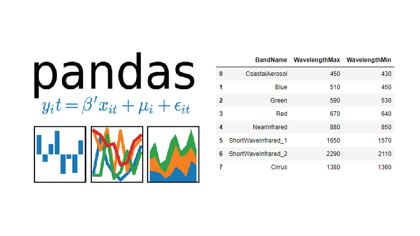
We used Pandas

Importing the data. Creating dataframes with Pandas methods. Using Pandas methods on our dataframes.

djia.dropna(axis=0, how='all', inplace=True)
djia.dropna(axis=1, how='any', inplace=True)
djia.isna().sum().sum()
----
for lag in range(1, lags + 1):
    col = f'lag_{lag}'
    djia_close[col] = djia_close['return'].shift(lag)
    cols.append(col)
djia_close.dropna(inplace=True)

djia_close.round(4).tail()

---

https://pandas.pydata.org/ Package overview pandas is a Python package providing fast, flexible, and expressive data structures designed to make working with “relational” or “labeled” data both easy and intuitive. It aims to be the fundamental high-level building block for doing practical, real-world data analysis in Python. Additionally, it has the broader goal of becoming the most powerful and flexible open source data analysis/manipulation tool available in any language. It is already well on its way toward this goal.

---

matplotlip

We used matplotlip

In creating statistical graphics The scatter methods to display correlations in our data. To plot detail It help fortifine our inital ideas in visual form.

fig, ax = plt.subplots(figsize=(10, 5))
plt.subplot(211)
plt.plot(Z)
plt.subplot(212)
plt.plot(returns);
----
plt.figure(figsize=(10, 6))
fig = plt.scatter(pvr[:, 0], pvr[:, 1],
                 c=psr, cmap='coolwarm')
cb = plt.colorbar(fig)
cb.set_label('Sharpe ratio')
plt.xlabel('expected volatility')
plt.ylabel('expected return')
plt.title(' | '.join(symbols))

---

https://matplotlib.org/ Matplotlib is a comprehensive library for creating static, animated, and interactive visualizations in Python.

• Plots created.

Timelaps plots of returns of test tickers

3d plot of expected volatility - expected return - sharpe ratio

bar plots of individual expected volatility - expected return - sharpe ratio values over time

---

Contributors

This project was created By Sam Prutton & Javier Barrios