Regularization is a very important technique in machine learning to prevent overfitting. Mathematically speaking, it adds a regularization term (penalty) in order to prevent the coefficients to fit so perfectly to overfit. The difference between the L1 and L2 is just that L2 is the sum of the square of the weights, while L1 is just the sum of the weights.
Regularization techniques in Generalized Linear Models (GLM) are used during a modeling process for many reasons. A regularization technique helps in the following main ways:
- Doesn’t assume any particular distribution of the dependent variable ( DV). The DV can follow any distribution such as normal, binomial, possison etc. Hence the name Generalized Linear Models (GLMs)
- Address Variance-Bias Tradeoffs. Generally will lower the variance from the model
- More robust to handle multicollinearity
- Better sparse data (observations < features) handling
- Natural feature selection
- More accurate prediction on new data as it minimizes overfitting on the train data
- Easier interpretation of the output

What is a regularization technique you may ask? A regularization technique is in simple terms a penalty mechanism which applies shrinkage (driving them closer to zero) of coefficient to build a more robust and parsimonious model. Although there are many ways to regularize a model, few of the common ones are:
- L1 Regularization aka Lasso Regularization– This add regularization terms in the model which are function of absolute value of the coefficients of parameters. The coefficient of the paratmeters can be driven to zero as well during the regularization process. Hence this technique can be used for feature selection and generating more parsimonious model
- L2 Regularization aka Ridge Regularization — This add regularization terms in the model which are function of square of coefficients of parameters. Coefficient of parameters can approach to zero but never become zero and hence
- Combination of the above two such as Elastic Nets– This add regularization terms in the model which are combination of both L1 and L2 regularization.
As the complexity is increasing, regularization will add the penalty for higher terms. This will decrease the importance given to higher terms and will bring the model towards less complex equation.
Ridge regression adds “squared magnitude” of coefficient as penalty term to the loss function. Here the highlighted part represents L2 regularization element.

Cost function
Here, if lambda is zero then you can imagine we get back OLS. However, if lambda is very large then it will add too much weight and it will lead to under-fitting. Having said that it’s important how lambda is chosen. This technique works very well to avoid over-fitting issue.
Lasso Regression (Least Absolute Shrinkage and Selection Operator) adds “absolute value of magnitude” of coefficient as penalty term to the loss function.

Cost function
Again, if lambda is zero then we will get back OLS whereas very large value will make coefficients zero hence it will under-fit.
The key difference between these techniques is that Lasso shrinks the less important feature’s coefficient to zero thus, removing some feature altogether. So, this works well for feature selection in case we have a huge number of features.
The difference between their properties can be promptly summarized as follows:
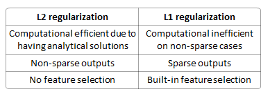
Built-in feature selection is frequently mentioned as a useful property of the L1-norm, which the L2-norm does not. This is actually a result of the L1-norm, which tends to produces sparse coefficients (explained below). Suppose the model have 100 coefficients but only 10 of them have non-zero coefficients, this is effectively saying that “the other 90 predictors are useless in predicting the target values”. L2-norm produces non-sparse coefficients, so does not have this property.
Sparsity refers to that only very few entries in a matrix (or vector) is non-zero. L1-norm has the property of producing many coefficients with zero values or very small values with few large coefficients.
Computational efficiency. L1-norm does not have an analytical solution, but L2-norm does. This allows the L2-norm solutions to be calculated computationally efficiently. However, L1-norm solutions does have the sparsity properties which allows it to be used along with sparse algorithms, which makes the calculation more computationally efficient.
The elastic net is a regularized regression method that linearly combines the L1 and L2 penalties of the lasso and ridge methods. The estimates from the elastic net method are defined by:

The quadratic penalty term makes the loss function strictly convex, and it therefore has a unique minimum. The elastic net method includes the LASSO and ridge regression: in other words, each of them is a special case where 


The elastic net method has been applied for Support Vector Machine.
Traditional methods like cross-validation, stepwise regression to handle overfitting and perform feature selection work well with a small set of features but these techniques are a great alternative when we are dealing with a large set of features.
[Source] https://medium.com/@jayeshbahire/lasso-ridge-and-elastic-net-regularization-4807897cb722
[Source] http://www.chioka.in/differences-between-l1-and-l2-as-loss-function-and-regularization/
[Source] https://towardsdatascience.com/l1-and-l2-regularization-methods-ce25e7fc831c
[Source] https://en.wikipedia.org/wiki/Elastic_net_regularization

