GithubHelp home page GithubHelp logo

bbrzycki / setigen Goto Github PK

View Code? Open in Web Editor NEW
25.0 1.0 12.0 78.43 MB

Python library for generating and injecting artificial narrow-band signals into radio frequency data

Home Page: https://setigen.readthedocs.io

License: MIT License

Jupyter Notebook 95.47% Python 4.53%
artificial-signals frequency signal-processing radio seti

setigen's Introduction

setigen

PyPI version AJ Paper Build Status Documentation Status codecov

setigen is a Python library for generating and injecting artificial narrow-band signals into radio frequency data, by way of data formats used extensively by the Breakthrough Listen (BL) team @ Berkeley.

Synthetic sine modulated signal + synthetic RFI signal

The main module of setigen is based on creating synthetic spectrogram (dynamic spectra) data, showing intensity as a function of time and frequency. Observational data saved in filterbank files can be loaded into setigen, and synthetic signals can be easily injected on top and saved out to file. setigen works well with file handling via BL's blimpy package.

The setigen.voltage module enables the synthesis of GUPPI RAW files via synthetic real voltage “observations” and a software signal processing pipeline that implements a polyphase filterbank, mirroring actual BL hardware. The voltage module supports single and multi-antenna RAW files, and can be GPU accelerated via CuPy.


Table of Contents

Installation

You can use pip to install the package automatically:

pip install setigen

Alternately, you can clone the repository and install it directly. At the command line, execute:

git clone [email protected]:bbrzycki/setigen.git
python setup.py install

The setigen.voltage module specifically can be GPU accelerated, via CuPy (https://docs.cupy.dev/en/stable/install.html). CuPy is not strictly required to use the voltage module, but it reduces compute time significantly. If CuPy is installed, enable setigen GPU usage either by setting the SETIGEN_ENABLE_GPU environmental variable to 1 or doing so in Python:

import os
os.environ['SETIGEN_ENABLE_GPU'] = '1'
os.environ['CUDA_VISIBLE_DEVICES'] = '0'

While it isn’t used directly by setigen, you may also find it helpful to install cusignal for access to CUDA-enabled versions of scipy functions when writing custom voltage signal source functions.

Spectrogram Format - setigen.Frame

Guiding Principles

Injecting an artificial signal is as simple as adding it to the data. To fully describe an artificial signal, we need the following:

  • Start and stop times (in most cases, this would probably be the beginning and end of the observation, assuming the signal is "on" continuously)
  • Frequency center of signal as a function of time sample
  • Intensity modulation of signal as a function of time sample
  • Frequency structure within each time sample
  • Overall intensity modulation as a function of frequency (bandpass)

setigen provides sample functions and shapes for each of these parameters. These all contribute to the final structure of the signal - the goal is to empower the user to generate artificial signals that are as simple or complex as one would like.

Minimal Working Example

Here's an example of synthetic signal generation, using astropy.units to express frame parameters:

from astropy import units as u
import setigen as stg
import matplotlib.pyplot as plt

frame = stg.Frame(fchans=1024,
                  tchans=32,
                  df=2.7939677238464355*u.Hz,
                  dt=18.253611008*u.s,
                  fch1=6095.214842353016*u.MHz)
noise = frame.add_noise(x_mean=10, noise_type='chi2')
signal = frame.add_signal(stg.constant_path(f_start=frame.get_frequency(index=200),
                                            drift_rate=2*u.Hz/u.s),
                          stg.constant_t_profile(level=frame.get_intensity(snr=30)),
                          stg.gaussian_f_profile(width=40*u.Hz),
                          stg.constant_bp_profile(level=1))

fig = plt.figure(figsize=(10, 6))
frame.plot()
plt.savefig('example.png', bbox_inches='tight')
plt.show()

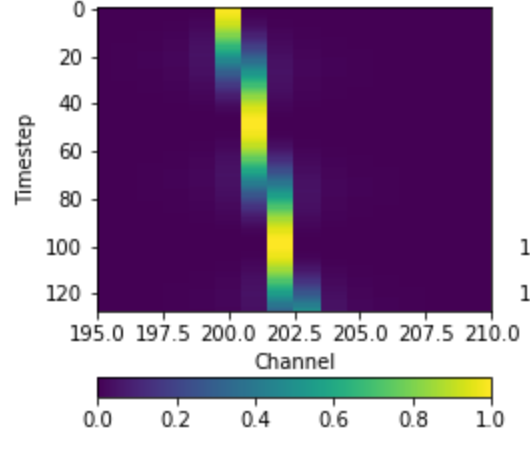
This first adds chi-squared noise to the frame, and adds a constant intensity signal at 30 SNR (relative to the background noise). The result is:

Example synthetic frame

Another example, using values found in real observations and visualized in the style of blimpy:

from astropy import units as u
import setigen as stg
import matplotlib.pyplot as plt

frame = stg.Frame(fchans=1024,
                  tchans=16,
                  df=2.7939677238464355*u.Hz,
                  dt=18.253611008*u.s,
                  fch1=6095.214842353016*u.MHz)
noise = frame.add_noise_from_obs()
signal = frame.add_signal(stg.constant_path(f_start=frame.get_frequency(index=200),
                                            drift_rate=2*u.Hz/u.s),
                          stg.constant_t_profile(level=frame.get_intensity(snr=30)),
                          stg.gaussian_f_profile(width=40*u.Hz),
                          stg.constant_bp_profile(level=1))

fig = plt.figure(figsize=(10, 6))
frame.plot()
plt.show()

Example obs synthetic frame

Cadences

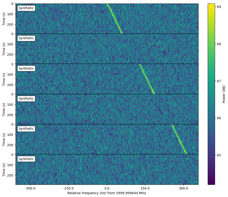
We can arrange a collection of frames as a setigen.Cadence object. This allows one to add noise and signals to multiple frames conveniently and to create publication-ready plots of observational cadences.

Cadence objects support list operations such as slicing and appending. This can be used to manage injection and analysis steps.

As a simple example with fully synthetic frames:

mjd_start = 56789
obs_length = 300
slew_time = 15

t_start_arr = [Time(mjd_start, format='mjd').unix]
for i in range(1, 6):
    t_start_arr.append(t_start_arr[i - 1] + obs_length + slew_time)
frame_list = [stg.Frame(tchans=16, fchans=256, t_start=t_start_arr[i]) 
              for i in range(6)]

c = stg.Cadence(frame_list=frame_list)
c.apply(lambda fr: fr.add_noise(4e6))
c[0::2].add_signal(stg.constant_path(f_start=c[0].get_frequency(index=128),
                                     drift_rate=0.2*u.Hz/u.s),
                   stg.constant_t_profile(level=c[0].get_intensity(snr=30)),
                   stg.sinc2_f_profile(width=2*c[0].df*u.Hz),
                   stg.constant_bp_profile(level=1),
                   doppler_smearing=True)
                            
fig = plt.figure(figsize=(10, 10))
c.plot()
plt.show()

Example synthetic cadence

Note that cadence objects don't have an imposed order -- they serve as a bare-bones organizational structure for frames. If you would like to impose an order, use the OrderedCadence:

c = stg.OrderedCadence(frame_list, 
                       order="ABACAD")

Ordered cadences additionally allow you to slice cadences by order label:

c.by_label("A")

If cadence frames are in chronological order, when plotting, you may spread subplots in the vertical direction proportionally to slew time with:

c.plot(slew_times=True)

Example synthetic cadence slew times

Raw Voltage Format - setigen.voltage

setigen.voltage block diagram

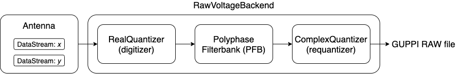
The setigen.voltage module extends setigen to the voltage regime. Instead of directly synthesizing spectrogram data, we can produce real voltages, pass them through a software pipeline based on a polyphase filterbank, and record to file in GUPPI RAW format. In turn, this data can then be reduced as usual using rawspec. As this process models actual hardware used by Breakthrough Listen for recording raw voltages, this enables lower level testing and experimentation. The basic layout of a setigen.voltage pipeline is shown above.

A simple example implementation may be written as follows. For more information, check out the docs.

from astropy import units as u
import setigen as stg

antenna = stg.voltage.Antenna(sample_rate=3e9*u.Hz,
                              fch1=6000e6*u.Hz,
                              ascending=True,
                              num_pols=1)

antenna.x.add_noise(v_mean=0,
                    v_std=1)

antenna.x.add_constant_signal(f_start=6002.2e6*u.Hz,
                              drift_rate=-2*u.Hz/u.s,
                              level=0.002)

digitizer = stg.voltage.RealQuantizer(target_fwhm=32,
                                      num_bits=8)

filterbank = stg.voltage.PolyphaseFilterbank(num_taps=8,
                                             num_branches=1024)

requantizer = stg.voltage.ComplexQuantizer(target_fwhm=32,
                                           num_bits=8)

rvb = stg.voltage.RawVoltageBackend(antenna,
                                    digitizer=digitizer,
                                    filterbank=filterbank,
                                    requantizer=requantizer,
                                    start_chan=0,
                                    num_chans=64,
                                    block_size=134217728,
                                    blocks_per_file=128,
                                    num_subblocks=32)

rvb.record(output_file_stem='example_1block',
           num_blocks=1,
           length_mode='num_blocks',
           header_dict={'HELLO': 'test_value',
                        'TELESCOP': 'GBT'},
           verbose=True)

A set of tutorial walkthroughs can be found at: https://github.com/bbrzycki/setigen/tree/main/jupyter-notebooks/voltage.

One unique application of the setigen.voltage pipeline is to ingest IQ data collected from an RTL-SDR dongle and create GUPPI RAW files accordingly: https://github.com/bbrzycki/rtlsdr-to-setigen.

setigen's People

Contributors

bbrzycki avatar radonnachie avatar

Stargazers

 avatar  avatar  avatar  avatar  avatar  avatar  avatar  avatar  avatar  avatar  avatar  avatar  avatar  avatar  avatar  avatar  avatar  avatar  avatar  avatar  avatar  avatar  avatar  avatar  avatar

Watchers

 avatar

setigen's Issues

Computation of noise stats should use `dtype=np.float64`

Computing the mean and std of large frames (e.g. ~16 million points) can suffer from floating point error when they are performed using float32 values. Both mean and std can be passed dtype=np.float64 to perform these computations using float64 instead and thereby retain better accuracy. One place where this could be added is here:

self.noise_mean, self.noise_std = np.mean(clipped_data), np.std(clipped_data)

but perhaps it would be good to add a dtype=np.float64 parameter to the enclosing function so that the user could specify a different type if desired.

Gist: using setigen to generate FRBs

I've been using setigen as a base to generate mock FRBs. Here's some example code:

def gauss2(x, a, x0, fwhm):
    """ Generate gaussian^2 pulse 
    
    Args:
        x: time series (np.arange())
        a: amplitude of pulse. (total integrated power across pulse)
        x0: index of peak value
        fwhm: width of signal in samples
    """
    sigma = (fwhm / 2) / np.sqrt(2*np.log(2))
    return a / np.sqrt(2*np.pi*sigma**2) * np.exp(-(x-x0)**2 / (2*sigma**2))


def generate_frb(frame, frb_params):
    """ Simple FRB generator 
    
    Args:
        frame (setigen.Frame): A filterbank frame of data, from setigen
        frb_params (dict): A dictionary with FRB parameters in it
        
    Notes:
        frb_params should contain width (in s), desired SNR, start time (in s), and DM
    """
    
    frb_width, frb_snr, frb_t0, frb_dm = frb_params['width'], frb_params['snr'], frb_params['t0'], frb_params['dm'], 

    frb_rms  = frame.get_intensity(snr=frb_snr)
    fch1 = frame.get_frequency(0)
    
    ## Generate pulse delays - array has same length as freqs
    width_in_chans = frb_width / frame.dt
    t0_in_samps = (frb_t0 / frame.dt) - frame.ts[0]
    tdel_in_samps = 4.15e-3 * frb_dm * ((fch1/1e9)**(-2) - (frame.fs/1e9)**(-2)) / frame.dt
    t0_in_samps = t0_in_samps + tdel_in_samps 
    
    # Time axis in samples
    t = np.arange(frame.tchans)

    # Use meshgrid to create (N_time, N_freq) array
    t2d, tdel2d = np.meshgrid(t, t0_in_samps)
    
    # Create pulse profile via 2D time (N_time,1) and time_delay (N_freq, 1) arrays
    profile = gauss2(t2d, frb_rms, tdel2d, width_in_chans)
    
    return profile.T

## Example usage
frame = stg.Frame(fchans=1024*u.pixel,
                  tchans=1024*2*u.pixel,
                  df=100.0*u.kHz,
                  dt=1*u.ms,
                  fch1=300*u.MHz)

noise = frame.add_noise(x_mean=10, noise_type='chi2')

frb_params = {'snr': 10000.0, 
              't0': 500e-3, 
              'dm': 3, 
              'width': 10e-3}
p = generate_frb(frame, frb_params)
frame.data += p

frb_params = {'snr': 10000.0, 
              't0': 1000e-3, 
              'dm': 10, 
              'width': 10e-3}
p = generate_frb(frame, frb_params)
frame.data += p

frame.plot()

Which gives the following output:

image

Just a proof of concept, but might be worth adding some functionality? This could be useful for FRB studies, and also for SETI seraches for artificial pulses (e.g. different exponents, negative DMs).

Error when trying to directly save extremely large frames

Example code:

frame = stg.Frame(fchans=2**24,
                  tchans=32,
                  df=1.3969838619232178*u.Hz,
                  dt=1.4316557653333333*u.s,
                  fch1=6095.214842353016*u.MHz)
frame.save_fil('test.fil')

This gives something like:

Traceback (most recent call last):
  File "/home/bryanb/setigen/setigen/frame.py", line 807, in save_fil
    self.waterfall.write_to_fil(filename)
  File "/home/bryanb/blimpy/blimpy/waterfall.py", line 317, in write_to_fil
    write_to_fil(self, filename_out)
  File "/home/bryanb/blimpy/blimpy/io/fil_writer.py", line 21, in write_to_fil
    __write_to_fil_heavy(wf, filename_out)
  File "/home/bryanb/blimpy/blimpy/io/fil_writer.py", line 50, in __write_to_fil_heavy
    bob = wf.container.read_blob(blob_dim, n_blob=ii)
  File "/home/bryanb/blimpy/blimpy/io/fil_reader.py", line 223, in read_blob
    blob = dd.reshape((int(dd.shape[0]/blob_dim[self.freq_axis]),blob_dim[self.beam_axis],blob_dim[self.freq_axis]))
ValueError: cannot reshape array of size 32768 into shape (0,1,24576000)

This might be some sort of interaction with blimpy Waterfall metadata.

IndexError: too many indices for array: array is 1-dimensional, but 3 were indexed

Expectation
The program below would run to conclusions without errors or it would clearly and consisely log a setigen limitation before throwing an exception.

Input file https://storage.googleapis.com/ata_test_data/turbo_seti_test/guppi_59196_68468_000762_Unknown_0001.rawspec.0000.h5

My program

import setigen as stg
from setigen.waterfall_utils import min_freq, max_freq
from blimpy import Waterfall

DIR = '/seti_data/turbo_seti_issue_135/'
INFILE = DIR + 'guppi_59196_68468_000762_Unknown_0001.rawspec.0000.h5'


def import_bl_file(path_infile):
    r'''
    Using setigen, import a BL file (.fil, .h5).
    '''
    print('Input file:', path_infile)
    wf = Waterfall(path_infile)
    print('Waterfall data loaded?', wf.container.load_data)
    print(wf.info())

    # Instantiate a setigen Frame object
    frame = stg.Frame(waterfall=wf)
    print('Drift rate:', frame.get_drift_rate(0, -1))
    print('Noise stats:', frame.get_noise_stats())
    print('min freq:', min_freq(wf))
    print('max freq:', max_freq(wf))

import_bl_file(INFILE)

Stdout

Input file: /seti_data/turbo_seti_issue_135/guppi_59196_68468_000762_Unknown_0001.rawspec.0000.h5
blimpy.io.base_reader WARNING  Selection size of 7.50 GB, exceeding our size limit 1.00 GB. Instance created, header loaded, but data not loaded, please try another (t,v) selection.

--- File Info ---
DIMENSION_LABELS :   ['time' 'feed_id' 'frequency']
        az_start :                              0.0
       data_type :                                1
            fch1 :                     8437.625 MHz
            foff :          1.9073486328125e-06 MHz
           ibeam :                               -1
      machine_id :                               20
          nbeams :                                1
           nbits :                               32
          nchans :                         33554432
            nifs :                                1
     rawdatafile : guppi_59196_68468_000762_Unknown_0001.0000.raw
     source_name :                          Unknown
         src_dej :                          0:00:00
         src_raj :                          0:00:00
    telescope_id :                               -1
           tsamp :                         2.097152
   tstart (ISOT) :          2020-12-13T19:01:08.000
    tstart (MJD) :                 59196.7924537037
        za_start :                              0.0

Num ints in file :                               60
      File shape :                (60, 1, 33554432)
--- Selection Info ---
Data selection shape :                (60, 1, 33554432)
Minimum freq (MHz) :                         8437.625
Maximum freq (MHz) :                8501.624998092651
None
Traceback (most recent call last):

  File "/home/elkins/seti_testing/blimpy_testing/stg_bug.py", line 24, in <module>
    import_bl_file(INFILE)

  File "/home/elkins/seti_testing/blimpy_testing/stg_bug.py", line 18, in import_bl_file
    frame = stg.Frame(waterfall=wf)

  File "/home/elkins/.local/lib/python3.8/site-packages/setigen/frame.py", line 120, in __init__
    self.data = waterfall_utils.get_data(self.waterfall)[:, ::-1]

  File "/home/elkins/.local/lib/python3.8/site-packages/setigen/waterfall_utils.py", line 75, in get_data
    return waterfall.data[:, 0, :]

IndexError: too many indices for array: array is 1-dimensional, but 3 were indexed

Support for NIFS > 1

It looks like @telegraphic is beginning significant work in blimpy to support multiple IFs (polarisation arrays) per time-integration. It would be very helpful to be able to generate Filterbank files as such using setigen.

Frame.save_h5|fil|hdf5 method, defaults defined kwargs, e.g. like tstart, in _update_waterfall method

As demonstrated in the cadences.ippynb in jupyter-notebooks/spectrogram, 6 frames are generated using the SETI ON/OFF cadence. I have saved these frames into 6 frame_0[0-5].h5 files and try to run it against turboSETI/plotSETI. The latter can not find hits using the plotSETI -f3 argument. This is caused by the fact the t_start of the frames are defaulted in the setigen Frame class by the "_update_waterfall" method. Though the t_start is provided as part of the Frame(... **kwargs), its value is defaulted in the mentioned method. This results into a wrong filterbank/h5 headers in the saved files. which do have all the same t_start times, hence plotSETI can not find hits.

Below the tstart times of the first 2 frames out of 6:

(hyperseti) marc@gamma2:~/tmp/test> watutil frame_00.h5 |grep tstart
   tstart (ISOT) :          2018-12-13T17:12:37.000
    tstart (MJD) :               58465.717094907406
(hyperseti) marc@gamma2:~/tmp/test> watutil frame_01.h5 |grep tstart
   tstart (ISOT) :          2018-12-13T17:12:37.000
    tstart (MJD) :               58465.717094907406

Sample code based on the jupyter notebook:

def create_time_array(cadence_number=6, mjd_start=60000, obs_length=300, slew_time=0):
    '''
    '''
    t_start_arr = [Time(mjd_start, format='mjd').unix]
    for i in range(1, cadence_number):
        t_start_arr.append(t_start_arr[i - 1] + obs_length + slew_time)   
    return t_start_arr

def create_frame(source_name, t_start, df, dt, obs_length):
    '''
    '''
    frame = stg.Frame(fchans=512,
                      tchans=int(obs_length/dt),
                      df=df,
                      dt=18.253611008,
                      fch1=1330*u.MHz,
                      ascending=False,
                      t_start=t_start,
                      source_name=source_name)        
    print(frame.t_start)
    return frame   

Plot of generated frames
setigen

TurboSETI cli log
For each HDF5 header, tstart is the same 'tstart': 58465.717094907406,
turbo_seti_cli.log

CAMRAS gitlab repo with used code
https://gitlab.camras.nl/seti/seti_dt_obs/-/blob/main/setigen/camras_gen.py

spectral kurtosis values of integrated chi-squared noise

I've been using spectral kurtosis for flagging in hyperseti, and have noticed that the noise statistics generated by setigen don't quite match what is expected from the generalized spectral kurtosis estimator, see:

The SK variance should come out as 2 / sqrt(N_accumulations) for a 'Pearson type IV' distribution, which I think most setigen generated data should be. I think this is just a matter of scaling the PDF by averaging first, but the math is admittedly a bit hectic in those papers.

Voltage notebook 03_custom_signals.ipynb produces errors with gpu (but not cpu)

The setigen voltage notebook 03_custom_signals.ipynb works fine for the cpu (os.environ['SETIGEN_ENABLE_GPU'] = '0') but produces an error with the gpu (os.environ['SETIGEN_ENABLE_GPU'] = '1') in the cell containing the rvb.record function. It appears that there is an issue with the time variable data type being converted to a numpy array. Cell error message is in pdf file included below. I don't have cusignal installed (deprecated?), so scipy.signal is being used.

03_custom_signals.ipynb with gpu error log.pdf

Error occurs in 06_starting_from_existing_raw_files.ipynb

In jupyter file 06_starting_from_existing_raw_files.ipynb, in the block calling stg.voltage.RawVoltageBackend.from_data(), that method appears to require a "digitizer" argument. This is the error message:

TypeError: RawVoltageBackend.from_data() missing 1 required positional argument: 'digitizer'

Is it just a matter of adding additional argument "digitizer=digitizer"? Is this then ignored in rvb.record() with the argument "digitize=False"?

Enhancement request: Need some help with the documentation!

The setigen utility is very interesting. Gave me some ideas for enhancing blimpy. Clearly, you put a lot of effort into it.

The documentation needs a review, in general:

  • Some items are 100% missing.
  • Some items do not explain the input parameters.
  • Some items need clarification for the audience.

E.g. setigen.stats module

All of the functions need explanation, including the input parameters.

I was wondering why there is no setigen.stats.get_max() since you have a get_min(). Just never had a need?

E.g. the Frame functions

Specifically, get_noise_stats() returns 2 floating-point numbers. Is that the mean noise and the standard deviation for the entirety of the time and frequency domains? How is this calculated.

How does get_total_stats() differ from get_noise_stats()?

The mean() and std() functions are based on what set of values? Signal power of the data in the frame?

render(use_db=False): if you are not plotting signal power values then what is the use_db= purpose?

render(): Frequency and time in pixels? I would have thought that MHz and seconds would be more convenient display for Seti BL folks. I might be missing something. Yes, I found bl_render() more interesting.

Doppler smearing support and scalloping loss question

Hey @bbrzycki, I'm working on some dedoppler efficiency tests, which brought up some setigen questions!

Firstly, how does setigen deal with signals with a drift rate larger than freq_resolution / time_resolution? (At first glance it didn't look like this was supported). The power for these will be spread over multiple channels causing 'smearing' and associated loss in S/N.

Secondly, I am realising that the FFT (or PFB) will affect how drifting signals manifest. A signal that starts in the middle of channel F0 will drift into channel F1, but there will be a period of time in which it is halfway between the two -- at which point it will actually appear in both channels, but at a lower S/N. There is also some 'scalloping loss' which occurs as the signal leaks across the full spectrum. Here's a simulation I did with a chirped waveform into an FFT filterbank:

image

(you can do better with an oversampled PFB).

To accurately evaluate dedoppler efficiency we would need to take both into account. I think doppler smearing would be straightforward to implement, but scalloping loss would be a bit of a nightmare -- and would depend on what kind of filterbank you had.

setigen crashes when large data arrays are required

It is impractical to download or even access every H5 or Filterbank file where trouble is reported. In order to investigate, it is highly desirable to be able to synthesize Filterbank files that resemble the file in question. E.g. a large data array file from observations of Tabby's Star (KIC8462852):

--- File Info ---
      machine_id :                               20
    telescope_id :                                6
       data_type :                                1
            fch1 :           19626.464842353016 MHz
            foff :      -2.7939677238464355e-06 MHz
          nchans :                        134217728
     source_name :                           maserA
         src_raj :                     20:39:29.112
         src_dej :                       11:12:59.4
        az_start :                              0.0
        za_start :                              0.0
           nbits :                               32
   tstart (ISOT) :          2016-12-19T20:44:33.000
    tstart (MJD) :               57741.864270833335
           tsamp :                     18.253611008
            nifs :                                1
Num ints in file :                                5
      File shape :                (5, 1, 134217728)
--- Selection Info ---
Data selection shape :                (5, 1, 134217728)
Minimum freq (MHz) :               19251.464845146984
Maximum freq (MHz) :               19626.464842353016

synthia.py.zip

To reproduce this issue, run the source file inside the attached ZIP file like this inside a terminal window:
python3 synthia.py

Linux reports: killed on an octacore with 16 GB RAM (mostly free).

Just change the value of the DIR variable to point to an output directory for saving the Filterbank file.
No other parameters needed.

Give get_intensity() an option to use statistics of time-integrated spectrum

get_intensity uses the statistics of the non-integrated frame to compute the intensity for a desired SNR. The involves dividing by the square root of the number of time samples in the frame, presumably to account for the sqrt(N) increase in the noise after integrating the time samples together. This is valid for purely noise-like signals, but for signals from "real" data the change in SNR after integration can be substantially different. The use of sigma clipping can further exacerbate this. The attached histograms of a frame real data from GBT shows how the standard deviation of the sigma trimmed pre- and post-integrated data can vary substantially (over 3x in this case).

Giving get_intensity an option to use the statistics of the time-integrated spectrum instead of the statistics of the flattened (and non-integrated) frame would be a welcomed addition.

image

Recommend Projects

  • React photo React

    A declarative, efficient, and flexible JavaScript library for building user interfaces.

  • Vue.js photo Vue.js

    🖖 Vue.js is a progressive, incrementally-adoptable JavaScript framework for building UI on the web.

  • Typescript photo Typescript

    TypeScript is a superset of JavaScript that compiles to clean JavaScript output.

  • TensorFlow photo TensorFlow

    An Open Source Machine Learning Framework for Everyone

  • Django photo Django

    The Web framework for perfectionists with deadlines.

  • D3 photo D3

    Bring data to life with SVG, Canvas and HTML. 📊📈🎉

Recommend Topics

  • javascript

    JavaScript (JS) is a lightweight interpreted programming language with first-class functions.

  • web

    Some thing interesting about web. New door for the world.

  • server

    A server is a program made to process requests and deliver data to clients.

  • Machine learning

    Machine learning is a way of modeling and interpreting data that allows a piece of software to respond intelligently.

  • Game

    Some thing interesting about game, make everyone happy.

Recommend Org

  • Facebook photo Facebook

    We are working to build community through open source technology. NB: members must have two-factor auth.

  • Microsoft photo Microsoft

    Open source projects and samples from Microsoft.

  • Google photo Google

    Google ❤️ Open Source for everyone.

  • D3 photo D3

    Data-Driven Documents codes.