brendancooley / icews-explorer

Shiny application for filtering, scaling, and visualizing dyadic event data from International Crisis Early Warning System (ICEWS)

ICEWS Explorer

Shiny application for filtering, scaling, and visualizing dyadic event data from International Crisis Early Warning System (ICEWS). To run:

require(shiny)
runGitHub("icews-explorer", user="brendancooley")

The application begins with raw event data. Each observation is a 'dyadic event', in which actor A takes some action X toward actor B on some date Y. The application performs 4 tasks:

1. Filter the raw event data.
2. Aggregate the data by dyad and time.
3. Scale the data to produce a low dimensional score for each dyad-time.
4. Visualize the data.

This document describes the data filtering and scaling procedures underlying the construction of the dynamic plots rendered in the application. Raw event data resides in the folder 'reducedICEWS' and was constructed using software developed by Phil Schrodt. The software converts the raw ICEWS files into a format suitable for analysis - associating each dyadic event with a source and target Correlates of War country code, a source and target sector (e.g. Government, Military, or Non-Governmental Organization), and event code (CAMEO and quad). Quad codes correspond to:

• 1: Verbal Cooperation
• 2: Material Cooperation
• 3: Verbal Conflict
• 4: Material Conflict

The script 'icewsReadr.R' processes the .txt files produced by the Schrodt software, stripping out events that have no country associated with them and events that occur within countries (self-dyads). The 'events.csv' file produced by this script lives in the repository and is also hosted on dropbox. It consists of ~7,100,000 dyadic events from 1995-2015. These are the data used by the application.

The application allows users flexibility in how they filter and scale this data.

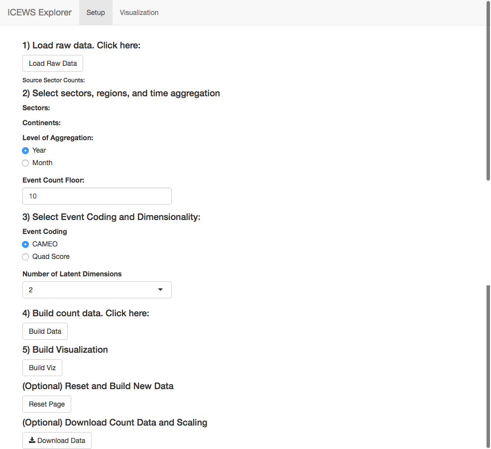
In the first step, users load the raw data. This can take a few minutes due to the size of the underlying event data. Once the data is loaded, a table of event counts by source sector is produced. In step 2, users filter and scale the data. Filtering can occur by continent and sector. For example, if only 'Africa' and 'GOV' are selected under 'Continents' and 'Sectors,' respectively, then only events that occured between governments in Africa will be included. In server.R,

# filter by sector
sectors <- input$sectors
continents <- input$continents
eventsSub <- filter(master$events0, sourceSec %in% sectors & tarSec %in% sectors & 
                    sourceContinent %in% continents & tarContinent %in% continents)

Then users choose how to aggregate the data. Data can be aggregated either by year or by month. If users choose to aggregate by year, the application converts the filtered event data into directed dyad-year-counts. Each row in the count data frame gives the number of events of each category that country A took toward country B in year Y. The 'Event Count Floor' field filters out dyad-years that experienced less than N events. Using N > 1 can improve the stability of the scaling algorithm, particularly when using the CAMEO event coding. The function event.counts() converts the filtered event data into count data.

event.counts <- function(events, agg.date, source, target, code) {
  counts <- events %>%
    group_by_(agg.date, source, target, code) %>%
    summarise(n = n()) %>%
    ungroup()
  output <- spread_(counts, code, 'n')
  output[is.na(output)] <- 0
  return(output)
}

This aggregated count data is used for analysis. The count data is difficult to analyze on its own. How should analysts distinguish more conflictual dyads from more cooperative ones? One solution is to simply count the number of conflictual events in a given time period and compare these counts across dyads. The problem with this approach is that dyads with high levels of interaction will have many events of all types, including conflictual events. To deal with this problem, analysts have developed conflict-cooperation scales, attaching a score to each event category and describing a dyad's conflict propensity with the average of it's event scores (see Goldstein 1994). While this solves the 'sum problem,' it induces a new 'mean problem.' A dyad that experiences 10 artillery barrages will receive the same score as a dyad which experiences a single artillery barrage, since artillery barrages have the same conflict-cooperation score.

A more satisfying alternative is to allow the data to produce the scale. Correspondence analysis (CA), which I employ here, is well suited to such scaling problems. The categorical corollary to principal components analysis, correspondence analysis first standardizes the count data, and then conducts a singular value decomposition on the residuals. This procedure converts the $N \times K$ matrix of "directed dyad time" by "event categories" into one $N \times M$ matrix and one $K \times M$ matrix, where $M$ is the number of latent dimensions (chosen by the user in the application). In our case, the $K \times M$ 'column matrix' tells us 'how much' of each event category a given dimension consists of. The $N \times M$ 'row matrix' tells us how each directed dyad time scores on each latent dimension. For example, if "material conflict" receives a high score on the first dimension in the column matrix, then dyads that experience relatively high amounts of material conflict should receive relatively high scores on this dimension in the row matrix. Substantive interpretation of the row coordinates depends on the values of the column coordinates and will vary based on which data are being used and how they are being aggregated. As Lowe shows, a 2-dimensional CA on quad count event categories seems to recover the Goldstein conflict-cooperation scale on the first dimension, and a material-verbal scale on the second dimension (see below).

See Greenacre 2016 for a full treatment of Correspondence Analysis and. I use Greenacre et al's ca library to implement the algorithm. The following code shows how the application converts the count data into scaled data.

# scale data
countData <- eCounts[,colnames(eCounts) %in% codes]
countData <- countData[,colSums(countData) > 0]
eCountsCA <- ca(countData, nd=input$ndim)
caBeta <- as_tibble(eCountsCA$rowcoord)
betas <- c()
for (i in 1:input$ndim) {
  betas <- c(betas, paste('beta', i, sep=""))
}
colnames(caBeta) <- betas
eCounts <- bind_cols(eCounts, caBeta)

# save column loadings to master
caGamma <- as_tibble(eCountsCA$colcoord)

caCol <- as_tibble(data.frame(colnames(countData), caGamma))

if (input$eCode == 'CAMEO') {
  colnames(caCol)[1] <- 'cameoCode'
  caCol <- left_join(caCol, cameoNames, by='cameoCode')
}
if (input$eCode == 'Quad Score') {
  colnames(caCol)[1] <- 'quadCode'
  caCol <- left_join(caCol, quadNames, by='quadCode')
}
master$colLoadings <- caCol

Once the data has been produced, users can either download it or proceed to the visualization on the second tab, an example of which is reproduced here:

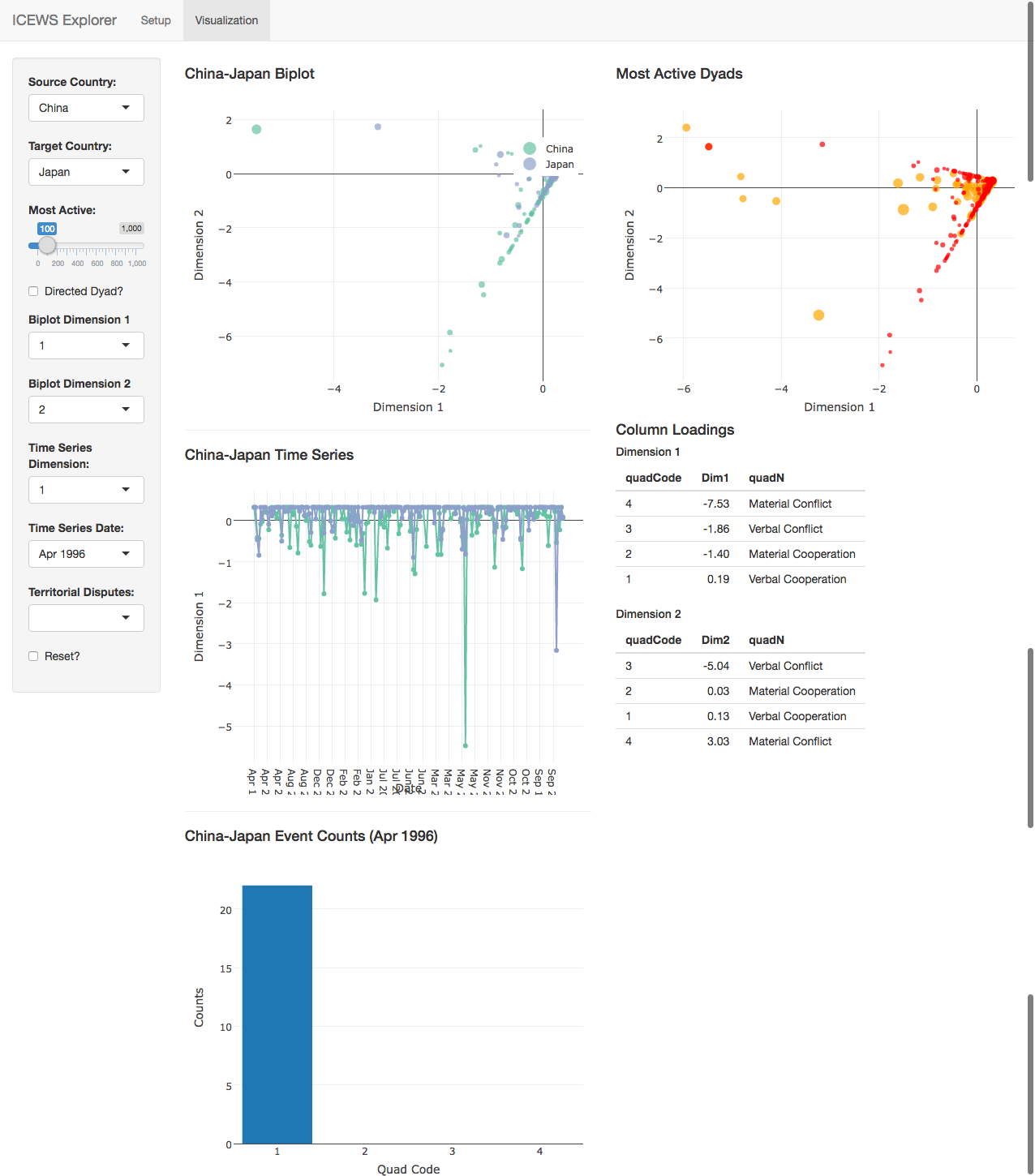
The file 'clAnalysis.R' conducts a brief analysis of the scalings produced by the correspondence analysis. It conducts a two-dimensional scaling of government-government events aggregated by year-month and categorized by quad score (verbal/material conflict/cooperation) for various event count floors. The column loadings produced by these scalings are reproduced here.

Dimension 1:

quadN	floor1	floor2	floor3	floor4	floor5	floor6	floor7	floor8	floor9	floor10
Verbal Cooperation	-0.2017274	-0.1947035	-0.1920362	-0.1915102	-0.1913303	-0.1923145	-0.1927148	0.1930594	0.1943069	0.1941384
Material Cooperation	3.0103006	2.0539494	1.7426425	1.6082685	1.5237554	1.4780429	1.4691721	-1.4494438	-1.4478242	-1.4006162
Verbal Conflict	2.1606949	2.1504111	2.0758776	2.0382932	1.9940767	1.9919117	1.9534699	-1.9063064	-1.9097470	-1.8559348
Material Conflict	7.5817133	7.8087666	7.8339917	7.8041390	7.7640850	7.7096856	7.6726670	-7.6251326	-7.5728805	-7.5338724

Dimension 2:

quadN	floor1	floor2	floor3	floor4	floor5	floor6	floor7	floor8	floor9	floor10
Verbal Cooperation	0.0387312	-0.1210403	0.1230214	0.1246692	0.1262031	0.1261990	0.1276886	0.1292959	0.1287924	0.1306992
Material Cooperation	-10.1848151	0.3907325	-0.1428822	-0.1667697	-0.1423416	-0.0927976	-0.0856832	-0.0560325	0.0289781	0.0347545
Verbal Conflict	0.7294221	5.0928095	-5.1174553	-5.1092452	-5.1041054	-5.0795993	-5.0679168	-5.0608281	-5.0411647	-5.0434213
Material Conflict	2.3445690	-3.6881863	3.4936377	3.4125436	3.3192515	3.3016508	3.2338664	3.1434710	3.1345373	3.0321333

The results show that the first dimension tends to distinguish cooperative from conflictual events, while the second dimension tends to distinguish verbal from material events. Note, however, that the scale sometimes flips. While conflictual events usually have negative values on the first dimensions, in some cases the most conflictual events take on positive values. The absolute values of the column loadings are relatively consistent, however, providing us with some confidence that the scaling algorithm is recovering a similar scale at each thresholds. Users should always check the column loadings before proceeding to analysis, to ensure that coefficients are interpreted properly.

References

Chang W, Cheng J, Allaire J, Xie Y and McPherson J (2017). shiny: Web Application Framework for R. R package version 1.0.3, <URL: https://CRAN.R-project.org/package=shiny>.

Wickham H, Francois R, Henry L and Müller K (2017). dplyr: A Grammar of Data Manipulation. R package version 0.7.2, <URL: https://CRAN.R-project.org/package=dplyr>.

Wickham H, Hester J and Francois R (2016). readr: Read Tabular Data. R package version 1.0.0, <URL: https://CRAN.R-project.org/package=readr>.

Wickham H (2017). tidyr: Easily Tidy Data with 'spread()' and 'gather()' Functions. R package version 0.6.3, <URL: https://CRAN.R-project.org/package=tidyr>.

Grolemund G and Wickham H (2011). “Dates and Times Made Easy with lubridate.” Journal of Statistical Software, 40(3), pp. 1-25. <URL: http://www.jstatsoft.org/v40/i03/>.

Sievert C, Parmer C, Hocking T, Chamberlain S, Ram K, Corvellec M and Despouy P (2017). plotly: Create Interactive Web Graphics via 'plotly.js'. R package version 4.7.0, <URL: https://CRAN.R-project.org/package=plotly>.

Zeileis A and Grothendieck G (2005). “zoo: S3 Infrastructure for Regular and Irregular Time Series.” Journal of Statistical Software, 14(6), pp. 1-27. doi: 10.18637/jss.v014.i06 (URL: http://doi.org/10.18637/jss.v014.i06).

Nenadic O and Greenacre M (2007). “Correspondence Analysis in R, with two- and three-dimensional graphics: The ca package.” Journal of Statistical Software, 20(3), pp. 1-13. <URL: http://www.jstatsoft.org>.

Gandrud C (2016). repmis: Miscellaneous Tools for Reproducible Research. R package version 0.5, <URL: https://CRAN.R-project.org/package=repmis>.

Arel-Bundock V (2017). countrycode: Convert Country Names and Country Codes. R package version 0.19, <URL: https://CRAN.R-project.org/package=countrycode>.

Xie Y (2017). knitr: A General-Purpose Package for Dynamic Report Generation in R. R package version 1.16, <URL: http://yihui.name/knitr/>.

Xie Y (2015). Dynamic Documents with R and knitr, 2nd edition. Chapman and Hall/CRC, Boca Raton, Florida. ISBN 978-1498716963, <URL: http://yihui.name/knitr/>.

Xie Y (2014). “knitr: A Comprehensive Tool for Reproducible Research in R.” In Stodden V, Leisch F and Peng RD (eds.), Implementing Reproducible Computational Research. Chapman and Hall/CRC. ISBN 978-1466561595, <URL: http://www.crcpress.com/product/isbn/9781466561595>.

Boettiger C (2017). knitcitations: Citations for 'Knitr' Markdown Files. R package version 1.0.8, <URL: https://CRAN.R-project.org/package=knitcitations>.

Francois R (2017). bibtex: Bibtex Parser. R package version 0.4.2, <URL: https://CRAN.R-project.org/package=bibtex>.