Data Science Path from Undergradate to Master

This repository store the notes about everything I learned from UoM Data Science Major and other online sources from 2019 to 2024. For me, this is more like a revision notes / cheatsheet for my future data science releated career.

If you notice something not so clear or errors or contents that confusing to other audiences, just start an issue and let's see what we can improve on it. Also, if there is a better way for categorisation, don't be hesitate starting a new issue! Let's make DS life more easier!

One thing I like to mention is although I may paraphrase some concept in my own words, sometimes I will directly copy past the concept from others' work. You can always find the original page just follow the reference page. Maybe the original content could give you a better understanding.

Notebooks
Reference

Mathematical Concepts

[Elaine & Johathan (2021)] Mathematics is the science that deals with the logic of shape, quantity and arrangement. Math is all around us, in everything we do. It is the building block for everything in our daily lives, including mobile devices, computers, software, architecture (ancient and modern), art, money, engineering and even sports.

Math Miscs

Probability

[Wikipedia] Probability theory is the branch of mathematics concerned with probability. Although there are several different probability interpretations, probability theory treats the concept in a rigorous mathematical manner by expressing it through a set of axioms. Typically these axioms formalise probability in terms of a probability space, which assigns a measure taking values between 0 and 1, termed the probability measure, to a set of outcomes called the sample space. Any specified subset of the sample space is called an event. Central subjects in probability theory include discrete and continuous random variables, probability distributions, and stochastic processes (which provide mathematical abstractions of non-deterministic or uncertain processes or measured quantities that may either be single occurrences or evolve over time in a random fashion). Although it is not possible to perfectly predict random events, much can be said about their behavior. Two major results in probability theory describing such behaviour are the law of large numbers and the central limit theorem.

Statistics

[Wikipedia] Statistics is the discipline that concerns the collection, organization, analysis, interpretation, and presentation of data. In applying statistics to a scientific, industrial, or social problem, it is conventional to begin with a statistical population or a statistical model to be studied. Populations can be diverse groups of people or objects such as "all people living in a country" or "every atom composing a crystal". Statistics deals with every aspect of data, including the planning of data collection in terms of the design of surveys and experiments.

Statistics is a mathematical body of science that pertains to the collection, analysis, interpretation or explanation, and presentation of data, or as a branch of mathematics. Some consider statistics to be a distinct mathematical science rather than a branch of mathematics. While many scientific investigations make use of data, statistics is concerned with the use of data in the context of uncertainty and decision making in the face of uncertainty.

Discrete Mathes and Operations Research: Linear Programming

Techniques of Operational Research

[Wikipedia] Operational research (OR) encompasses the development and the use of a wide range of problem-solving techniques and methods applied in the pursuit of improved decision-making and efficiency, such as simulation, mathematical optimization, queueing theory and other stochastic-process models, Markov decision processes, econometric methods, data envelopment analysis, neural networks, expert systems, decision analysis, and the analytic hierarchy process.[5] Nearly all of these techniques involve the construction of mathematical models that attempt to describe the system. Because of the computational and statistical nature of most of these fields, OR also has strong ties to computer science and analytics. Operational researchers faced with a new problem must determine which of these techniques are most appropriate given the nature of the system, the goals for improvement, and constraints on time and computing power, or develop a new technique specific to the problem at hand (and, afterwards, to that type of problem).

Voting Methods

[Wikipedia] Voting is a method for a group, such as a meeting or an electorate, in order to make a collective decision or express an opinion usually following discussions, debates or election campaigns. Democracies elect holders of high office by voting. Residents of a place represented by an elected official are called "constituents", and those constituents who cast a ballot for their chosen candidate are called "voters". There are different systems for collecting votes, but while many of the systems used in decision-making can also be used as electoral systems, any which cater for proportional representation can only be used in elections.

Voting Criteria
- Mutual Majority
- Monotonicity
- Participation
- Independence of irrelevant alternatives
- Later no harm
Plurality voting
Majority judgement
Instant runoff voting
Multiple Rounds voting
Condorcet Voting
Borda count
Score voting

Machine Learning

[Wikipedia] Machine learning (ML) is a field of inquiry devoted to understanding and building methods that 'learn', that is, methods that leverage data to improve performance on some set of tasks.[1] It is seen as a part of artificial intelligence. Machine learning algorithms build a model based on sample data, known as training data, in order to make predictions or decisions without being explicitly programmed to do so.[2] Machine learning algorithms are used in a wide variety of applications, such as in medicine, email filtering, speech recognition, and computer vision, where it is difficult or unfeasible to develop conventional algorithms to perform the needed tasks.

Dimensionality Reduction Methods

[Wikipedia] Dimensionality reduction, or dimension reduction, is the transformation of data from a high-dimensional space into a low-dimensional space so that the low-dimensional representation retains some meaningful properties of the original data, ideally close to its intrinsic dimension. Working in high-dimensional spaces can be undesirable for many reasons; raw data are often sparse as a consequence of the curse of dimensionality, and analyzing the data is usually computationally intractable (hard to control or deal with). Dimensionality reduction is common in fields that deal with large numbers of observations and/or large numbers of variables, such as signal processing, speech recognition, neuroinformatics, and bioinformatics.

Feature selection

[Wikipedia] Feature selection approaches try to find a subset of the input variables (also called features or attributes). The three strategies are: the filter strategy (e.g. information gain), the wrapper strategy (e.g. search guided by accuracy), and the embedded strategy (selected features are added or removed while building the model based on prediction errors).

Data analysis such as regression or classification can be done in the reduced space more accurately than in the original space.

Feature projection

[Wikipedia] Feature projection (also called feature extraction) transforms the data from the high-dimensional space to a space of fewer dimensions. The data transformation may be linear, as in principal component analysis (PCA), but many nonlinear dimensionality reduction techniques also exist.[4][5] For multidimensional data, tensor representation can be used in dimensionality reduction through multilinear subspace learning.

Dimension reduction

[Wikipedia] For high-dimensional datasets (i.e. with number of dimensions more than 10), dimension reduction is usually performed prior to applying a K-nearest neighbors algorithm (k-NN) in order to avoid the effects of the curse of dimensionality.[20]

Feature extraction and dimension reduction can be combined in one step using principal component analysis (PCA), linear discriminant analysis (LDA), canonical correlation analysis (CCA), or non-negative matrix factorization (NMF) techniques as a pre-processing step followed by clustering by K-NN on feature vectors in reduced-dimension space. In machine learning this process is also called low-dimensional embedding.[21]

For very-high-dimensional datasets (e.g. when performing similarity search on live video streams, DNA data or high-dimensional time series) running a fast approximate K-NN search using locality-sensitive hashing, random projection, "sketches", or other high-dimensional similarity search techniques from the VLDB conference toolbox might be the only feasible option.

Evaluation Metrics

Wrapper Methods

Embeded Methods

Ensemble Learning

Data Processing Concepts

Supervised Learning Methods

Unsupervised Learning Methods

Neural Network

Activation Functions

Artificial Intelligence

[Wikipedia] Artificial intelligence (AI) is intelligence demonstrated by machines, as opposed to the natural intelligence displayed by animals including humans. AI research has been defined as the field of study of intelligent agents, which refers to any system that perceives its environment and takes actions that maximize its chance of achieving its goals.

The term "artificial intelligence" had previously been used to describe machines that mimic and display "human" cognitive skills that are associated with the human mind, such as "learning" and "problem-solving". This definition has since been rejected by major AI researchers who now describe AI in terms of rationality and acting rationally, which does not limit how intelligence can be articulated.

Four Approaches to defining AI

Thinking like a human
- figure out how we think by introspection or experimentation (cognitive modeling).
- self-awwareness is important: "I think therefore I am".
- Humans feel emotions and apparently don't always think (or act) rationally.
Thinking rationally
- problem is how do we define rationality, this could be defined via logic since logic has greatly influenced AI.
Acting like a human
Acting rationally
- The rational agent: perform actions which will (most likely) achieve one's goals.
A rational agent acts to maximize the expectation of the performance measure, conditioned on the percept sequence to date, and whatever built-in knowledge the agent posseses.

"It is a branch of computer science by which we can create intelligent machines which can behave like a human, think like humans, and able to make decisions." (Java T Point)

Goals of Artifical Intelligence

Replicate human intelligence
Solve knowledge-intensive tasks
An intelligent connection of perception and action
Building a machine which can perform tasks that requires human intelligence such as:
- Proving a math theorm
- Play chess game
- Plan some surgical operation
- Self-driving a car
Creating some system can exhibit intelligent behavior, learn new things by itself, demonstrate, explain, and can advise to its user.

Advantages of Artificial Intelligence	Disadvantages of Artificial Intelligence
High accuracy with less error	High cost
High-speed	Can't think out of the box
High reliability	No feelings and emotions
Useful for risky areas	Increase dependency on machines
Digital Assistant	No original creativity
Useful as a public utility

Artificial Intelligence Types

Based on Capabilities	Based on functionality
Weak AI / Narrow AI	Reactive Machines
General AI	Limited Memory
Super AI	Theory of Mind
	Self-Awareness

Intelligent Agent

An agent is any entity which perceives and acts in an environment. The percept sequence is defined as the complete history of content the agent has perceived. Agent behaviour is defined by an agent function mapping the given percept sequence to an action. An agent program is responsible for implementation the agent function within some physical system.

We evaluate agent behavior through the performance measure. A rational agent acts to maximize the expectation of the performance measure, conditioned on the percept sequence to date, and whatever built-in knowledge the agent possesses.

A self-learning agent may undertake actions to modify future percepts, and/or adjust the agent function as it accumulates experience.

Types of Agent

Agent Architectures
Agents can be grouped into five classes based on their degree of perceived intelligence and capability. All these agents can improve their performance and generate better action over the time. These are given below:
- Simple reflex agent：only chooses actions based on the current percept, and ignores all preceding information.
- Model-based reflex agent：maintains some internal state which depends on the percept history, useful if the current environment cannot be fully described by the current percept.
- Goal-based agents：makes decisions in order to achieve a set of predefined goals, in addition to maintaining internal state. In practice usually superceded by utility-based agent.
- Utility-based agent：compares the desirability of different environment states via a utility function. This allows the comparison of different goal states and action sequences and tradeoffs between different goals.
- Learning Agent: can learn from its past experiences or it has learning capabilities. It starts to act with basic knowledge and then is able to act and adapt automatically through learning.
Agent model: charaterise requirements for an agent in terms of its percepts, actions, environment and performance measure.

Agent types: choose and justify choice of agent type for a given problem.

Environment types: characterise the environment for a given problem.
Questions [True/False]
- An agent that senses only partial information about the state cannot be perfectly rational.
  - FALSE
  - Rationality refers to optimality of decisions according to some performance measuer conditioned upon the evidence provided by the percept sequence, in addition to whatever prior knowledge it has.
- There exist task environments in which no pure reflex agent can behave rationally.
  - TRUE
  - Pure reflex agents cannot maintain a history of past actions/percepts, so nay environment where optimality erquires conditioning on the previous state(s) satisfies this criterion.
- Suppose an agent selects its action uniformly at random from the set of possible actions. There exists a deterministic task environment in which this agent is rational.
  - TRUE
  - Consider the situation where all actions taken yield the same rewards.
- An agent which chooses the action with the highest expected value under the performance measure is superior to all other agents in the long run.
  - 'Highest expected value' was left deliberately ambiguous as a discussion point.
  - TRUE
    - If we assume this references to maximization of the total cumulative performance measure in the future, then the agent is optimal by definition.
  - FALSE
    - If this instead refers to immediate reward observed at each stage, choosing the action with the highest expected value at the current timestep is greedy, and may be suboptimal, as aficionados of dynamic programming can attest
    - Sometimes it is necessary to sacrifies immediate reward for long-term optimality.
- Every agent is rational in an unobservable environment.
  - FALSE
  - It is possible to build in prior knowledge into an agent about acceptable behaviour in the absense of observations. An agent lacking this prior knowledge may take suboptimal actions in unobservable environment.
Intelligent Agent

Any agent composed with four parts:
- Percepts: percepts or observations of the environment, made by sensors
- Actions: which affect the environments, made actuators
- Environment: where the agent exist
- Performance measure: performance measurement evaluate the desirability of environment states
In short, an agent can be anything that perceiveits environment through sensors and act upon that environment through actuators. An Agent runs in the cycle of perceiving, thinking, and acting.

An AI system can be defined as the study of the rational agent and its environment. The agents sense the environment through sensors and act on their environment through actuators. An AI agent can have mental properties such as knowledge, belief, intention, etc.
Questions
- Do agent functions exist which cannot be implemented by any agent program? If yes, give a counterexample.
  - Yes
  - if the agent function rquires solving an undecidable problem - e.g. suppose the agentfunction required one to solve a Diophantine equation or decide wheter an arbitrary Turing machien halts. THen there is no agent program capable of implementing this agent function.
- Suppose we keep the agent program fixed but speed up the machine by a factor of two. Does this change the agent function? Will your answer change depending on the environment type?
  - Depends on the program and the environment
    - Dynamic environment
      
      It speedup may allow the agent to act sonner to choose different, better actions.
    - Static environment
      
      the agent function is unchanged, only speedup the processing speed.
Agent Environment

An environment is everything in the world which surrounds the agent, but it is not a part of an agent itself. An environment can be described as a situation in which an agent is present.

The environment is where agent lives, operate and provide the agent with something to sense and act upon it. An environment is mostly said to be non-feministic.

Environment Properties
- Fully/partially observable: The environment is fully observable if the agent's sensors capture the complete state of the environment at every point in time. Imperfect sensors/models or a fundamental inability to capture environmental state lead to partial observability.
- Single/multi agent: Self explanatory, although care must be taken in deciding which entities in the environment mustbe considered fellow agents.
- Deterministic/stochastic: if future states of the environment is a special case of a nondeterministic environment which admits a probabilistic model of environment phenomena.
- Episodic/sequential: If an agent's percept sequence is divided into noninteracting episodes, where the agent executes a single action based on the current percept, the environment is episodic. In a sequential environment, the current action may affect future environment state and hence future decisions.
- Static/Dynamic:If the environment can change when the agent is deliberating (executing the agent program), then the environment is dynamic, otherwise static.
- Discrete/continuous: If the environment has a finite number of distinct states, then the agent only has to contend with a finite set of percepts, and the environment is discrete, otherwise continuous. Similarly, if an agent can choose between a finite number of actions, the action set is discrete.
Questions

For each of the following activities, characterize the task environment in terms of its properties:
- Playing soccer
  - Partially observable, stochastic, sequential, dynamic, continous, multi-agent
- Shopping for used books on the internet
  - Partially observable, deterministic, sequential, static, single agent.
  - This can be multi-agent and dynamic if we buy books via auction, or dynamic if we purchase on a long enough scale that book offers change.
- Bidding on an item at an auction
  - Fully observable, stochastic (assuming non-rational actors), sequential, static, discrete, multi-agent.
Turing Test in AI

Turing Test was introduced by Alan Turing in his 1950 paper, "Computing Machinery and Intelligence", which considered the question, "Can Machine think?"

Problem with Truing test:
Turing test is not reproducible, constructive or amenable to mathematical analysis.

Problem-solving

# Problem solving agent
funtion SIMPLE-PROBLEM-SOVING-AGENT(p) returns an action
    inputs: p, a perception of the current environment
    static: s, an action sequence, initially empty
            state, some description of the current world state
            g, a goal, initially null
            problem: a problem formualation
    
    state <- UPDATE-STATE(state, p)
    
    if s is empty then
        g <- FORMULATE-GOAL(state)
        problem <- FORMULATE-PROBLEM(state, g) # need to define the states and operators
                                               # state is described as how the agent store the perceived information
                                               # for example, to let a robot move to some point, we need to know 
                                               #              the current robot coordinates, e.g. robot joint angle. or
                                               #              to solve a 8 puzzle, the board state is represented by the 
                                               #              the integer location of the tile
                                               
        s <- SEARCH(problem)

    # find valid, optimal, rational actions
    action <- RECOMMENDATION(s, state)
    s <- REMAINER(s, state)
    
    return action

Search Algorithms

Search algorithms are one of the most important areas of Artificial Intelligence. This topic will explain all about the search algorithms in AI.

Basic idea: offline, simulated exploration of state space by generating successors of already-explored states (a.k.a. expanding states).
```
function GENERAL-SEARCH(problem, strategy) returns a solution, or failure
    initialize the search tree using the initial state of problem
    
    loop do
        if there are no candicates for expansion then return failure
        
        choose a leaf node for expansion according to strategy
            if the node contains a goal state then return the corresponding solution
            else expand the node and add the resulting nodes to the search tree
    end

# implementation

function GENREAL-SEARCH(problem, QUEING-FN) returns a solution or failure
    nodes <- MAKE-QUEUE( MAKE_NODE(INITIAL-STATE[problem]) )
    loop do
        if nodes is empty then return failure
        
        node <- REMOVE-FRONT(nodes) # since the QUEUE is a priority queue, always pop the first node
        if GOAL-TEST[problem] applied to STATE(node) succeeds then return node
        nodes <- QUEUING-FN( nodes, EXPAND(node, OPERATIONS[problem]) )
                                    # EXPAND function creates new nodes, filling in various fields and using OPERATORS (or ACTIONS) of problem to create the corresponding states.
    end
```
States vs. Nodes
- A state is a (representation of) a physical configuration.
- A node is a data structure constituting part of a search tree includes parent, children, depth, path, cost g(x).
States do not have parents, children, depth, or path cost.
Questions
- In BFS and DFS, an undiscovered node is marked discovered when it is first generated, and marked processed when it has been completely searched. At any given moment, several nodes might simultaneously be in the discovered state.
  - Describe a graph on n vertices and root v such that Θ(n) nodes are simultaneously in the discovered state when conducting BFS starting from v.
    - A graph of depth 1 where v has n children, the tree becomes a list where the search time will be Θ(n)。
  - Repeat the above question, but for DFS.
    - A graph of depth n with a single linear branch of children extending from v. In this case the tree will be a stick.
  - Describe a graph on n vertices and root v such that at some point Θ(n) remain undiscovered, while Θ(n) nodes have been processed during DFS starting from v.
    - A graph of depth n/2 with two linear equal-length branches of children extending from v. Note the case in the second question is not acceptable here as any node along the chain is not marked processed util the recursion returns.
- Recall the iterative deepening search (IDS) strategy
  - Derive the time complexity of iterative deepening search on a graph with branching factor b and minimum goal depth d.
    - Within each iteration, IDS exhaustively enumerates all nodes up to the current depth. At depth n, the size of this set is b^n, Nodes at all levels apart from d are re-generated multiple-times.
    - The node in the penultimate layer are generated twice, the nodes in the third-last layer are genereted three times, and so on, with the root node generated d times. This implies that an upper bound on the number of generated nodes, and hence the time complexity is:
      
      d + (d + 1)b + (d + 2)b^2 + ... + 2d^{d-1} + b^d = O(b^d). So asymptotically approaches to BFS.
  - Can you think of a situation where IDS performs much worse than regular depth-first search?
    - Consider the situation where the graph is a linear chain with depth d. DFS terminates in d iteration but IDS takes \sum^d_{n=1} n(n+1)/2 iterations.
  - BFS and IDS are not optimal in general. State a necessary condition on the cost function g : paths → R for both methods to be optimal.
    - Necessary for g to be a non-decreasing function of depth - otherwise the cost of a path from the start to the goal state could be decreased by taking a path with a greater number of actions. This can be formally proved via induction.
- A graph G = (V,E) is connected if a path exists between any two vertices v1,v2 ∈ V. A connected component of a graph is a maximal subset Vc ⊆ V such that there exists a path between any two vertices in Vc. Describe an algorithm, using graph search, that accepts an arbitrary graph G as input and counts the number of connected components of G.
  - For undirected graphs with a finite state space, BFS/DFS will eventually enumerate all vertices within a connected component, starting at an arbitrary node within the connected component, since the vertex ordering is irrelevant:
    - Start at an arbitrary node.
    - Run BFS/DFS until the frontier is exhausted - all proceesed vertices belong to the first connected component.
    - Restart BFS/DFS from an arbitrary undiscovered node until all vertices have been marked processed, counting the number of restarts time.
- Your tutor’s job is to arrange n ill-behaved children in a straight line, facing front. They are given a list of m statements of the form "child i hates child j". If i hates j, they cannot put i somewhere behind j, because i is then capable of throwing something at j.
  - They have enlisted your help to design an algorithm which orders the line (or says it is not possible), using depth-first search. Analyze the running time of your algorithm.
    - From a directed graph with the vertices corresponding to children and an edge pointing from i to j if j hates i.
    - Topologically sort the graph as follows:
      
      Form a stack which will hold the topologically sorted nodes.
      
      Perform DFS, and push nodes σ onto stack only after all descendants of σ in the graph have been fully explored/processed. If there is an edge i -> j, this guarantees that i is only pusehd onto the stack after j.
      
      The top node on the stack always has no incoming edge from any vertex in the stack.
      
      Repreatedly popping nodes off the stack yields a topological ordering where i will always precede j if j hates i.
  - For the class photo, the children must be arranged in rows such that if i hates j, i must be in a lower-numbered row than j, otherwise it is possible for i to drop something on j. Design an efficient algorithm to find the minimum number of rows needed.
    - Construct the graph as before. The seating position of children not involved in a hate relation are irrelevant (these represent singleton disconnected nodes), so we want to find the height of the connected component of the graph of maximum height. This can be found in O(m+n) time using BFS to enumerate all vertices within each connected components.
Uniform Search Algorithm

Uninformed search is a class of general-purpose search algorithms which operats in brute-force way. Uninformed search algorithms do not have additional information about state or search space other than how to traverse the tree, so it is also called blind search.
Heuristic Function

Heuristic is a function which is used in Informed Search, and it finds the most promising path. It takes the current state of the agent as its input and produces the estimation of how close agent is from the goal. The heuristic method, however, might not always give the best solution, but it guaranteed to find a good solution in reasonable time. Heuristic function estimates how close a state is to the goal. It is represented by h(n), and it calculates the cost of an optimal path between the pair of states. The value of the heuristic function is always positive.

*Admissbility of the heuristic function is given as: h(n) <= h(n).

Here h(n) is heurstic cost, and h*(n) is the estimated cost. Hence heuristic cost should be less than or equal to the estimated cost.

Admissibnle heuristics can be derived from the exact solution cost of relaxed version of the problem.
- For example, if the rules of the 8-puzzle are relaxed so that a tile can move anywhere then h1(n) gives the shortest solution.
  - h1(n) = number of misplaced tiles
  - h2(n) = total Manhattan distance
- If the rules are relaxed so that a tile can move to any adjacent square, then h2(n) gives the shortest solution.
h(σ) ≤ min(cost(σ → goal)) = h*(σ), ∀σ ∈ Σ

An admissible heuristic defines an optimal cost estimate; it never overestimate the cost to the goal. Note sacrificing admissibilty does not completely void the heuristic function - you lose guarantees of optimality, but non-admissible heuristics may allow you search method to run faster as less nodes in the priority queue need to be expanded - in general there is a tradeoff between speed/optimality.

Consistency/Monotony

h(σ) ≤ cost(σ, σ′,A) + h(σ′) ∀σ ∈ Σ, A(σ) = σ′

This is the triangle inequality applied to costs of graph states. Here cost(σ, σ′,A) denotes the cost to the agent of taking action A in state σ to end up in state σ′.

Admissibility results in optimality but may not be completeness in general.
Informed Search Algorithm

Informed Search algorithms have information on the goal state which helps in more efficient searching. This information is obtained by a function that estimates how close a state is to the goal state (Geeks for Geeks, 2021).
Questions
- Suppose that we run a greedy best-first (graph) search algorithm with the heuristic function for node σ set to the negative of the path cost, h(σ) = −g(σ). What sort of search will the greedy search emulate?
  - This emulates depth-frist search, noting that for froniter F: argmin f(σ) = argmax(σ).
- The heuristic path algorithm is a best-first search where the evaluation function contains a relative weighting factor w: f(σ) = (2 −w)g(σ) + wh(σ).
  - What kind of search does this perform for w = 0, w = 1, and w = 2?
    - w = 0: uniform cost search
    - w = 1: A* search
    - w = 2: Gready Best First Search
  - For what values is it optimal, assuming that the heuristic h is admissible? Hint: recall the condition for optimality of A∗.
    - Note that f(σ) = (2 - w)(g(σ) + w / (2 - w) h(σ)), a scaled version of A* with heuristic w/(2-w)h(σ). We require this to be admissible, hence require w / (2-w) ≤ 1 ⇒ w ≤ 1. Non-negativity of the heuristic requires then 0 ≤ w ≤1.
- Recall that state generation refers to the creation of thedata structure σ representing the state, whereas state expansion refers to the generation ofall children of the present node.
  - Should informed search algorithms apply the goal test upon state generation or state expansion, in order for the resulting search to be optimal? Does it make a difference from uninformed search algorithms?
    - Apply the goal test on generation does not guarantee optimality in general for informed search methods (and UCS).
    - There may be lower-cost paths living in the frontier which we have not explored.
    - However if we apply the goal test on expansion, all nodes in the frontier will have equal or larger path cost. For uniformed search algorithms (except UCS) this dose not affect optimality but will affect time complexity. For example, BFS time complexity becomes O(b^{d+1}) for goal test upon expansion.
- n vehicles occupy squares (1,1) through (n,1) (i.e., the bottom row) of an n×n grid. The vehicles must be moved to the top row but in reverse order; so the vehicle i that starts in (i,1) must end up in (n −i + 1,n). On each time step, every one of the n vehicles can move one square up, down, left, or right, or stay put; but if a vehicle stays put, one other adjacent vehicle (but not more than one) can hop over it. Two vehicles cannot occupy the same square.
  - Find an expression for the size of the state space in terms of n.
    - n^2! / (n^2 - n)!
  - Find an expression for the branching factor in terms of n.
    - 5^n
  - Give a (non-trivial) admissible heuristic h_i for the number of moves it takes for a single vehicle i starting in (xi,yi) to its goal state, (n −i + 1,n). Manhattan Distance
  - Is \sum_i h_i an admissible heuristic for this problem? How about max{h1,...,hn} or min{h1,...,hn}?
    - The first will not be admissible general as vehicles can move simultaneously. Note for the 'hop' operation one vehicle must remain and other jump 2 steps, meaning the toal distance travelled by all cars per move is bounded above by n. The total distance D moved by all vehicles from the start to goal state is bounded below by n min{h_1,...,h_n} ≤ D. Hence the minimum number of steps requird to attain D is min{h_1,...,h_n}.

Uninformed Search vs. Informed Search (Geeks for Geeks, 2021)

Uninformed Search	Informed Search
It doesn't use knowledge for searching process	It uses knowledge for the searching process
It finds solution slow as compared to informed search	It finds solution more quickly
It is always complete	It may or may not be complete
Cost is high	Cost is Low
It consumes moderate time	It consumes less time
No suggestion is given regarding the solution in it	It provides the direction regarding the solution
It is more lengthy while implementation	It is less lengthy while implementation
DFS, BFS, DLS, UCS, IDDFS	Best-First search, A* search

Hill Climbing Algorithm

Hill climbing algorithm is a local search algorithm which continuously moves in the direction of increasing elevation/value to find the peak of the mountain or best solution to the problem. It terminates when it reaches a peak value where no neighbor has a higher value.

Hill climbing algorithm is a technique which is used for optimizing the mathematical problems. One of the widely discussed examples of Hill climbing algorithm is Traveling-salesman Problem in which we need to minimize the distance traveled by the salesman.

It is also called greedy local search as it only looks to its good immediate neighbor state and not beyond that.

A node of hill climbing algorithm has two components which are state and value.

Hill Climbing is mostly used when a good heuristic is available.

In this algorithm, we don't need to maintain and handle the search tree or graph as it only keeps a single current state.
```
function HILL-CLIMBING(problem) returns a solution state
    inputs: problem
    local variables: current, a node
                     next, a node
    current <- MAKE-NODE(INITIAL-STATE[problem])
    loop do
        next <- a highest-valued successor of current
        if VALUE[next] < VALUE[current] then return current
        current <- next
    ends
```
The problem of hill-climbing algorithm is it can get stuck on local maxima.
Means-Ends Analysis

Means-Ends Analysis is problem-solving techniques used in Artificial intelligence for limiting search in AI programs. It is a mixture of Backward and Forward search technique. The MEA process centered on the evaluation of the difference between the curernt state and goal state.

Summary Search Stragies/Algorithm Properties

A strategy is defined by picking the order of node expansion. Strategies are evaluated along the following dimensions: completeness, time complexity, space complexity, optimality.

Time complexity calculate number of nodes generated/expanded.
Space complexity calculate maximum number of nodes in memeory.
Completeness evaluate is the strategy/algorithm always find a solution if one exist.
Optimality evaluate is the strategy/algorithm always find a least-cost solution.

	Time Complexity	Space Complexity	Completeness	Optimality Comparisons
(Uninformed Search) Breadth-first search	O(b^d)	O(b^d)	Complete	Optimal
(Uninformed Search) Depth-first search	O(n^m)	O(bm)	Complete	Non-optimal
(Uninformed Search) Depth-limited search	O(b^ℓ)	O(bℓ)	Complete if solution is above ℓ	Non-optimal
(Uninformed Search) Uniform cost search	O(b^{1+[C*/ε]})	O(b^{1+[C*/ε]})	Complete if there is a solution	Optimal
(Uninformed Search) Iterative deepening depth-first search	O(b^d)	O(bd)	Complete if branching factor is finite	Optimal if path cost is a non-decreasing function of depth of the node
(Uninformed Search) Bidirectional search	O(b^d)	O(b^d)	Complete	Optimal if both search use BFS
(Informed Search) Best-First search	O(b^m)	O(b^m)	Incomplete	Non-optimal
(Informed Search) Greedy search	O(b^m)	O(b^m)	Incomplete	Non-optimal
(Informed Search) A* search	O(b^d)	O(b^d)	Complete if finite branching factor & fixed cost	Optimal if heuristic functions is admissible and consistency

d = depth of shallowest solution
b = branching factor, a node at every state
m = maximum depth of any node
ℓ = depth limit parameter

Problem formulation usually requires abstracting away real-world details to define a state space that can feasibly be explored.
There are lots of variety of uniformed search strategies.
Iterative deepening search uses only linear space and not much more time than other uninformed search algorithms.
Heuristics help reduce search cost, however, finding an optimal solution is still difficult.
Greedy best-first is not optimal but can be efficient.
A* search is complete and optimal but is prohibitive in memory.
Hill-climbing methods operate on complete-state formulations, requires less memeory, but not optimal.

Adversarial Search

Adversarial Search

Adversarial search is a search, where we examine the problem which arises when we try to plan ahead of the world and other agents are planning against us.

Usually, a game will have an unpreditable opponent and time limits for play. Thus our agent should use adversarial search find solution with a form contingency plan and approaximate the best solution in time bounds.

Types of Games: game types could be described as the following table.

Deterministic Chance

Perfect information chess
checkers
go
othello backgammon
monopoly

Imperfect information bridge
poker
scrable
nuclear war

Games illustrate seveval important points about AI.
- perfection is unattainable => must approximate and make trade-offs
- uncertainty limits the value of look-ahead
- programs could use TDLearning (self-learning agent) to learn the game from past game experience or using supervised learning like gradient decent search to find the best solution.
  - problems
    - Delayed reinforcement: reward resulting from an action may not be received until several time steps later, which also slows down the learning.
    - Credit assignment: need to know which action(s) was responsible for the outcome.
Minimax Search

Minimax is a perfect play for deterministic, perfect-information games.

Minimax algorithm is a recurisive or backtracking algorithm which is used in decision making and game theory. It provides an optimal move for the player assuming that opponent is also playing optimally. Minimax algorithm uses recursion to search through the game-tree. Minimax algorithm is mostly used for game playing in AI. Such as Chess, Checkers, tic-tac-toe, go, and various two-players game. This algorithm compute the minimax decision for the current state. In this algorithm, two players play the game, one called MAX and other is called MIN. Both the players fight it as the opponent player gets the minimum benefit while they get the maximum benefit. Both Players of the game are opponent of each other, where MAX will select the maximized value and MIN will select the minimized value. The minimax algorithm performs a depth-first search algrotihm for the exploration of the comlete game tree. The minimax algorithm proceeds all the way down to the terminal node of the tree, then backtrack the tree as the solution.
```
function MINIMAX-DECISION(game) returns an operator
    for each op in OPERATIONS[game] do
        VALUE[op] <- MINIMAX_VALUE( APPLY(op, game), game )
    end
    return the op with the highest VALUE[op]

function MINIMAX-VALUE(state, game) returns a utility value
    if TERMINAL-TEST[game](state) then
        return UTILITY[game](state)
    else if MAX is to move in state then
        return the highest MINIMAX-VALUE of SUCCESSORS(state)
    else if MIN is to move in state then
        return the lowest MINIMAX-VALUE of SUCCESSORS(state)
```
Properties of minimax algorithm
- Complete: Minimax algorithm is complete, it will definitely find a solution (if exist) in the finite search tree.
- Optimal: Minimax algorithm is optimal if both opponent are player optimally.
- Time complexity: As it performs DFS for the game-tree, so the time complexity of minimax algorithm is O(b^m), where b is branching factor of the game-tree, and m is the maximum depth of the tree.
- Space complexity: Space complexity of minimax algorithm is aslo similar to DFS which is O(bm).
In the real world, usually there is a resouce limits for minimax algorithm. For example a player has limited time or there is not enough computational power for successors exploration. What we can do is using two approaches:
- cutoff test: e.g. depth limit (perhaps add quiescence search)
  
  MINIMAX-CUTOFF is identical to MINIMAX-VALUE except we add depth limit as an additional terminal check, and using utility function to replace the evaluation function.
- evaluation fucntion = estimated desirability of position These two approach are effective to shortern the time complexity and space complexity of minimax search.
Limitation of the minimax algorithm:
- The main drawback of the minimax algorithm is that it gets really slow for complex games such as Chess, go, etc. This type of games has a huge branching factor, and the player has lots of choices to decide. This limitation of the minimax algorithm can be improved from alpha-beta pruning.
Alpha-beta Pruning

Alpha-beta pruning is a modified version of the minimax algorithm. It is an optimization technique for the minimax algorithm. As we have seen in the minimax search algorihtm that the number of game states it has examine are exponential in depth of the tree. Since we cannot eliminate the exponent, but we can cut it to half. Hence there is a technique by which without chekcing each node of the game tree we can compute the corerct minimax decision, and this technique is called pruning. This involves two threshold parameter Alpha and Beta for future expansion, so it is called alpha-beta pruning. It is also called Alpha-Beta Algorithm. Alpha-beta pruning can be applied at any depth of a tree, and sometimes it not only prune the tree leaves but also entire sub-tree. The two-parameter can be defined as:
- Alpha: The best (highest-value) choice we have found so far at any point along the path for maximier. The initial value of alpha is -inf.
- Beta: The best (lowest-value) choice we have found so far at any point along the path for minimier. The initial value of beta is inf.
The alpha-beta pruning is a standard minimax algorithm returns the same move as the standard algorithm does, but it removes all the nodes which are not really affecting the final decision but making algorithm slow. Hence by pruning these node, it makes the algorithm fast.

Alpha-beta pruning is a modified version of the minimax algorithm. It is an optimization technique for the minimax algorithm.
```
function MAX-VALUE(state, game, α, β) returns the minimax value of state
    inputs: state, current state in game
            game, game description
            α, the best score for MAX along the path to state
            β, the best score for MIN along the path to state

    if CUTOFF-TEST(state) then return EVAL(state)
    for each s in SUCCESSORS(state) do
        α <- MAX(α, MIN-VALUE(s, game, α, β))
        if α >= β then return β
    end
    return α
    
function MIN-VALUE(state, game, α, β) returns the minimax value of state
    if CUTOFF-TEST(state) then return EVAL(state)
        β <- MIN(β, MAX-VALUE(s, game, α, β))
        if β <= α then return α
    end
    return β
```
Pruning does not affect final reulst.

The order of search nodes is important in alpha-beta pruning. If we have the worst-ordering, the time complexity will be exactly the same as minimax O(b^m). However, if we have an ideal ordering, then the time complexity will reduce in half since the best node always on the left side of the tree, complexity will be O(b^{m/2}). As a result, the agent could doubles depth of search.
Questions
- Here you will investigate the fundamentals of minimax and alpha- beta pruning. Consider noughts and crosses on a 3 ×3 grid. Define Xn as the number of rows, columns or diagonals with exactly n crosses and no noughts. Define On analogously. Assume our utility function assigns +1 to any position with X3 = 1 and −1 to any position with O3 = 1, with all other positions having zero utility. For nonterminal positions, use the evaluation function f(s) = 3X_2(s) + X_1(s) −(3O_2(s) + O_1(s)) . Assume the cross player goes first.
  - Find an (possibly approximate) expression for the size of the state space in terms of n, i.e. how many possible configurations exist.
    - b = 9, m = 9, naively obvious bounds are 9^9, 9! or 3^9. Note number of possible games > number of unique states as a game consider state ordering.
  - Construct the whole game tree starting with an empty board down to depth 2 (i.e., one X and one O on the board), taking symmetry into account. Mark the evaluations of all positions at depth 2.
    - Root has a minimax value of +1
    - At depth of 1, MIN encounters the following values:
      
      X at top left: -1
      
      X at top mid: -2
      
      X at centre: +1
    - Continuous
  - Use minimax to mark the backed-up values for the positions at depth 1, and use these values to choose the optimal move for the X player.
    - See above
  - Circle the nodes at depth 2 that would not be evaluated if alpha-beta pruning was applied, assuming the nodes were generated in the optimal order for alpha-beta pruning.
    - In total, 8 of the 12 leaf nodes ca nbe pruned by alpha-beta with optimal move ordering.
- Why is minimax less reasonable than expectiminimax as a practical decision-making principle for a complex agent acting in the real world?
  - The real world is often stochastic and in complex environments with inherent randomness it is generally necessary to use probability distribution to parameterize our uncertainty.
  - More practically, minimax assumes an optimal adversary - it is more likely that optimal responses to an agent's actions are not guaranteed.
  - Minimax makes decisions based on the potentially low-probability worst case scenario.
  - Recall that expectiminimax uses the expected utility over its children. This weights events and their corresponding outcomes according to their probability in the expectation, so may be more robust to higly negative but very rare events.
- The minimax algorithm returns the best move for MAX under the assumption that MIN plays optimally. What happens when MIN plays suboptimally?
  - Assertion: For every game tree, the utility obtained by MAX using minimax decisions against a suboptimal MIN will be never be lower than the utility obtained playing against an optimal MIN.
    - Consider a MIN node whose children are terminal nodes. For a suboptimal opponent, the utility of the node is greater or equal than the value than if MIN played optimally, U(σ_min) >= U*(σ_min).
    - Hence ther value of the parent MAX node, which assumes the maximum among all it's children, is greater than the ase for an optimal MIN player.
    - Repeat this argument until the root node and conclude that the assertion is ture, the max player always enjoys payoff greater or equal to the case of an optimal MIN player.
- Minimax and alpha-beta as presented assume a zero-sum setting with boundedutility functions. This question prompts you to consider the consequences of removing theseassumptions.
  - Describe how the minimax and alpha–beta algorithms change for two-player, non-zero-sum games in which each player has a distinct utility function and both utility functionsare known to both players.
    - For non-zero sum games between two players A and B, a single value is not sufficient to describe the utility of a node, and should instead be replaced by a tuple of vaelus (v_A, v_B), giving the minimax value/utility of the state for each respective player. At each stage the player whose turn it is to move selects the action that yeilds the highest v_i value.
    - Alpha-beta pruning is not possible in this context as the game is not necessaryily adversial and the two players are not necessarily copmeting against each other - the utility functiosn may be entirely independent, and neither player may be particularly fussed about what the other player does. There may no longer be situations where one player will never let the other player down a particular branch of the game tree.
  - What happens in the almost cooperative case, where the utility functions differ by atmost a positive constant k > 0, i.e. UA = UB + k?
    - The optimal strategy in this scenario is for both players to cooperate to reach the maximum-valued leaf - the agents work together to achieve a mutually desirable goal.
Temporal Difference Learning (TDLeaf(λ))

Temporal difference (TD) learning refers to a class of model-free reinforcement learning methods which learn by bootstrapping from the current estimate of the value function. These methods sample from the environment, like Monte Carlo methods, and perform updates based on current estimates, like dynamic programming methods.

While Monte Carlo methods only adjust their estimates once the final outcome is known, TD methods adjust predictions to match later, more accurate, predictions about the future before the final outcome is known (Wikipedia, 2022).

From above, we know supervised learning is for sinlge step prediction, but Temporal Difference (TD) leraning is for multi-step prediction.
- Correctness of prediction not known until several steps later
- Intermediate steps provide information about correctness of prediction
- TD learning is a form of reinforcement learning
TDLeaf(λ) algorithm combines temporal difference learning with minimax search, the basic idea is update weight in evaluation function to reduce differences in rewards predicted at different levels in search tree. Good functions should be stable from one move to next.

Notations
- eval(s, w): evaluation function for state s with parameters w = [w_1, ..., w_k]
- s_1, ..., s_N: the N states that occurred during a game
- r(S_N): reward based on outcome of game {+1, 0, -1}
- s_i^l: best leaf found at max cut-off depth using minimax search starting at state s_i
To convert evaluation score into a reward, we could using r(s_i^l, w) = tanh(eval(s_i^l, w)) where tanh squashes the evaluation score into the range [-1, +1].
```
# Algorithm

For i = 1, ..., N-1 Compute temporal difference between successive states
    d_i = r(s_{i+1}^l, w) - r(s_i^l, w)

Update each weight parameter w_j as follows
    w_j <- w_j + \eta \sum^{N-1}_{i=1} \partial r(s_i^l, w) / \partial w_j [\sum^{N-1}_{m=1} λ^{m-i}d_m]
where \eta is the learning rate

if λ = 0: weights adjusted to move r(s_i, w) towards r(s_{i+1}, w)
    i.e. the predicted reward at the next state
if λ = 1: weights adjusted to move r(s_i, w) towards r(s_N)
    i.e. the final true reward (better if eval() is unrealistic)
```
By using the reinforcment learning in game play, with a large number of games experience, the probability of taking a move that leads to a loss should go to zero, and the probability of taking a move that leads to a win should approach to 1, so that the agent will favor the optimal action. This assumes taht every move in every possible state has been visited sufficiently many times so that we can obtain a viable estimate of its usefullness.
Questions

Recall for a general state s, and parametric evaluation function Eval(s; θ) we would like Eval(s; θ) ≈ U(s), where U(s) is the backed-up utility of the terminal state that arises from playing the game out from state s, using minimax up to depth l with the evaluation function Eval for both players.

We have to play s out to completion in order to make a single weight update based on s. But playing out s to completion generates multiple intermediate states {s_t,s_{t+1},...,s_N} that we may use to refine our weight updates.
- Assume the objective function is ℓ(θ; s) = 1/2 (U(s) −Eval(s; θ))^2. Show that the gradient descent weight update from playing a state s until completion is: θ ←θ + η (U(s) −Eval(s; θ)) ∇_θ Eval(s; θ).
```
This follows from the chain rule:
    ∇_θ ℓ(θ; s) = −∇_θ Eval(s; θ)(U(s) −Eval(s; θ))
Subtitute into the update rule θ ← θ −η∇_θ ℓ(θ; σ) to obtain the result.
```
- By using minimax with depth l to look ahead, we only calculate rewards from states of depth l in the future. If sl is the state whose reward ultimately propagates back to s via minimax, the weight update rule is: θ ← θ + η U(s) −Eval(s^l; θ)∇_θEval(s^l; θ) To be clear, here Eval(sl; θ) is the evaluation obtained for state s by applying Eval to the leaf nodes of a depth l minimax search from s. The weight update rule tries to make Eval(s_l; θ) a good approximation to the true terminal utility. If {s_t,s_{t+1},...,s_N} are the states encountered in a training game starting at time step t, we define the evaluation function at the terminal state s_N as the utility of s_t. The contribution to the parameter update by passing through state s_t is θ ←θ + η Eval(s^l_N; θ) −Eval(s^l_t; θ)∇_θ Eval(s^l_t; θ). Show the total update to the parameter vector for all N −1 moves made from state s_1 is: θ ← θ + η \sum^{N-1}_{i=1} Eval(s^l_N; θ) − Eval(s^l_i; θ)∇_θ Eval(s^l_i; θ).
```
The parameter update for all N - 1 is the sum of all incremental updates ∆θ_t due to passing through states s_t:
    θ ← θ + \sum^{N−1}_{t=1} ∆θ_t
      = θ + η\sum^{N-1}_{t=1} Eval(s^l_N; θ) −Eval(s^l_i; θ) ∇_θ Eval(s^l_i; θ)
```
- Finally, we note that Eval(s_N; θ) −Eval(s^l_i,θ) is a telescoping series: Eval(slN; θ) −Eval(sli; θ) = \sum^{N-1}+{m=1} Eval(s^l_{m+1}; θ) −Eval(s^l_m; θ) Define the temporal differences d_m = Eval(s^l_{m+1}; θ) −Eval(s^l_m; θ). Show the update rule reduces to: θ ←θ + η\sum^{N-1}{i=1} (∇_θ Eval(s^l_i; θ) \sum^{N-1}{m=i}d_m).
  - Straight forward from the definitions.
- We can insert a decay term λ ∈[0,1] which controls the effect of this telescoping: θ ← θ + η\sum^{N-1}{i=1} (∇_θ Eval(s^l_i; θ) \sum^{N-1}{m=i} λ^{m-i}d_m). This is the final update rule for TDLeaf(λ). Identify the update rules for the λ = 0 and λ = 1 cases, how does the behaviour of the updates qualitatively change as we increase λ?
```
For λ = 0, (noting that lim_{x→0^+}x_0 = 1), only m = i term in the inner sum is non-zero, and the update looks like:
    θ ← θ + η\sum^{N-1}_{t=1} ∇_θ Eval(s^l_t; θ)[Eval(s^l_t+1; θ) −Eval(s^l_t; θ)]
This is known as the one-step temporal difference update, training is guided to minimize the change in reward between consecutive status.

For λ = 1, the telescope collapses to yield:
    θ ← θ + η\sum^{N-1}_{t=1} ∇_θ Eval(s^l_t; θ)[U(s) −Eval(s^l_t; θ)]
Here training is being guided to miniumize the difference between each state's s_t predicted reward with the final state's utility at time step N. This is equivalent to gradient descent using only terminal state utilities as targets.
Setting 0 < λ < 1 controls how far into the future the algorithm should look ahead in determining its update. Increasing λ interpolates between the short-sighted one-step λ = 0 behavior and the long-sighted λ = 1 behavior.
```
Monte Carlo Search Tree

In computer science, Monte Carlo tree search (MCTS) is a heuristic search algorithm for some kinds of decision processes, most notably those employed in software that plays board games. In that context MCTS is used to solve the game tree.

MCTS is an algorithm that figures out the best move out of a set of moves by Selecting → Expanding → Simulating → Updating the nodes in tree to find the final solution. This method is repeated until it reaches the solution and learns the policy of the game (SAGAR, 2018).
Backtracking

Backtracking refers to a general method of building sequence of decisions to solve a graph problem incrementally. Suppose we have a partial solution to a problem we would like to extend: A = (a_1, a_2, ..., a_k). To choose next solution component, a_{k+1}:
- Recursively evaluate every possible consistent with past decisions. When we establish that a partial solution cannot be extended into a complete solution, or is worse than the current best solution, we terminate the recursive call, thereby pruning regions of state space from the search tree which cannot contain a solution (or an optimal solution if we have some notion of optimality). We backtrack to the deepest node with unexpanded children and invoke recursion again.
- Choose a valid successor (or the 'best' one if we have optimality criterion), A ←A \cup a+{k+1}. Repeat until A becomes a complete solution.
This implmented as depth-frist/recursive traversal with additional logic at each call that helps narrow the search space, using problem constraints to prune subtrees as early as possible.
```
def backracking_dfs(A, k):
    if A = (a_1, a_2, ..., a_k) in solution:
        return A
    else:
        k += 1
        
        # enumerate all possible candidates extending deepest partial solution
        candidate_queue = construct_candidates(A, k)
        
        # while valid children exist, extend solution by recursion
        while candidate_queue is not None:
            A[k] = candidate_queue.pop() # add current candidate to A
            result = backtrack_dfs(A, k)
            
            if result != failure:
                return result
            A[k] = null # backtrack, remove candidate from A
    return failure
```

	Deterministic	Chance
Perfect information	chess checkers go othello	backgammon monopoly
Imperfect information		bridge poker scrable nuclear war

Knowledge Represent

Knowledge Based Agent

An intelligent agent needs knowledge about the real world for taking decisions and reasoning to act efficiently. Knowledge-based agents are those agents who have the capability of maintaining an internal state of knowledge, reason over that knowledge, update their knowledge after observations and take actions. These agents can represent the world with some formal representation and act intelligently.

Knowledge-based agents are composed of two main part:
- Knowledge-base
- Inference system
A knowledge-based agent must able to do the following:
- An agent should be able to represent states, actions, etc.
- An agent should be able to incorporate new percepts
- An agent can update the internal representation of the world
- An agent can deduce the internal representation of the world
- An agent can deduce appropriate actions
Knowledge Representation

Humans are best at understanding, reasoning, and interpreting knowledge. Human knows things, which is knowledge and as per their knowledge they perform various actions in the real world. But how machines do all these things comes under knowledge representation and reasoning. Hence we can describe Knowledge representation as following:
- Knowledge representation and reasoning (KR, KRR) is the part of Artificial intelligence which concerned with AI agents thinking and how thinking contributes to intelligent behavior of agents.
- It is responsible for representing information about the real world so that a computer can understand and can utilize this knowledge to solve the complex real world problems such as diagnosis a medical condition or communicating with humans in natural language.
- It is also a way which describes how we can represent knowledge in artificial intelligence. Knowledge representation is not just storing data into some database, but it also enables an intelligent machine to learn from that knowledge and experiences so that it can behave intelligently like a human.
Knowledge Representation Techniques

There are mainly four ways of knowledge representation which are given as follows:
- Logical representaiton
- Semantic Network Representation
- Frame Representation
- Production Rules
Propositional Logic

Propositional logial (PL) is the simplest form of logic where all the statements are made by propositions. A proposition is a declarative statement which is either true or false. It is a technique of knowledge representation in logical and mathematical form.
Rules of Inferece

In artificial intelligence, we need intelligent computers which can create new logic from old logic or by evidence, so generating the conclusions from evidence and facts is termed as inference.
Example of Knowledge-Based Agent
- The Wumpus world
- Knowledge-base for Wumps World
First-order logic

First-order logic is another way of knowledge representation in artificial intelligence. It is an extension to propositional logic. FOL is sufficiently expressive to represent the natural language statements in a concise way. First-order logic also known as Predicate logic or First-order predicate logic. First order logic is a powerful language that develops information about the objects in a more easy way and can also express the relationship between thoese objects. First-order logic (like natural language) does not only assume that the world contains facts like propositional logic but also assumes the following things in the world:
- Objects: A, B, people, numbers, colors, wards, theories, squares, pits, ...
- Relations: It can be unary reltaion such : red, round, is adjacent, or n-any relation such as: the sister of, the brother of, has color, comes between, ...
- Functions: Father of, best friend, third inning of, end of, ...
As a natural language, first-order logic also has two main parts:
- Syntax
- Semantics
Knowledge Engineering in FOL

The process of constructing a knowledge-base in first-order logic is called as knowledge- engineering. In knowledge-engineering, someone who investigates a particular domain, learns important concept of that domain, and generates a formal representation of the objects, is known as knowledge engineer.
Inference in First-order logic

Inference in First-Order Logic is used to deduce new facts or sentences from existing sentences. Before understanding the FOL inference rule, let's understand some basic terminologies used in FOL.
Unification in FOL

Unification is a process of making two different logical atomic expressions identical by finding a substitution. Unification depends on the substitution process. It takes two literals as input and makes them identical using substitution. Let Ψ1 and Ψ2 be two atomic sentences and 𝜎 be a unifier such that, Ψ1𝜎 = Ψ2𝜎, then it can be expressed as UNIFY(Ψ1, Ψ2).
Resolution in FOL

Resolution is a theorem proving technique that proceeds by building refutation proofs, i.e., proofs by contradictions. It was invented by a Mathematician John Alan Robinson in the year 1965.

Resolution is used, if there are various statements are given, and we need to prove a conclusion of those statements. Unification is a key concept in proofs by resolutions. Resolution is a single inference rule which can efficiently operate on the conjunctive normal form or clausal form.
Forward Chaining and Backward Chaining

In artificial intelligence, forward and backward chaining is one of the important topics, but before understanding forward and backward chaining lets first understand that from where these two terms came.

Forward Chaining vs. Backward Chaining

Forward Chaining	Backward Chaining
Forward chaining starts from known facts and applied inference rule to extract more data unit it reaches to the goal	Backward chaining starts from the goal and works backward through inference rules to find the required facts that support the goal
It is a bottom-up approach	It is a top-down approach
Forward chaining is known as data-driven inference technique as we reach to the goal using the available data	Backward chaining is known as a goal-driven technique as we start from the goal and divide into sub-goal to extract the facts
Forward chaining reasoning appplies a breadth-first search strategy	Backward chaining reasoning applies a depth-frist search strategy
Forward chaining tests for all the available rules	Backward chaining only tests for few required rules
Forward chaining is suitable for the planning, monitoring, control, and interpretation application	Backward chaining is suitable for diagnostic, prescription, and debugging application
Forward chaining can generate an infinite number of possible conclusions	Backward chaining generates a finite number of possible conclusions
It operates in the forward direction	It operates in the backward direction
Forward chaining is aimed for any conclusion	Backward chaining is only aimed for the required data

Reasoning in AI

The reasoning is the mental process of deriving logical conclusion and make predictions from available knowledge, facts, and beliefs. Or we can say, "Reasoning is a way to infer facts from existing data." It is a general process of thinking rationally, to find valid conclusions.

Inductive vs. Deductive Reasoning

Basis for comparison	Deductive Reasoning	Inductive Reasoning
Definition	Deductive reasoning is the form of valid reasonin, to deduce new information or conclusion from known related facts and information	Inductive reasoning arraives at a conclusion by the process of generalization using specific facts or data
Approach	Deductive reasoning follows a top-down approach	Inductive reasoning follows a bottom-up approach
Starts from	Deductive reasoning starts from premises	Inductive reasoning starts from conclusion
Validity	In deductive reasoning conclusion must be true if the premises are true	In inductive reasoning, the truth of premises does not guarantee the truth of conclusions
Usage	Usage of deductive reasoning is difficult, as we need facts which must be true	Use of inductive reasoning is fast and easy, aswe need evidence instead of true facts. We othen use it in our daily life
Process	Thoery -> Hypothesis -> Patterns -> Confirmation	Obserations -> Patterns -> Hypothesis --> Theory
Argument	In deductive reasoning, arguments may be valid or invalid	In inductive reasoning, arguments may be weak or strong
Structure	Deductive reasoning reaches from general facts to specific facts	Inductive reasoning reaches from specific facts to general facts

Uncertain Knowledge R

Probabilistic Reasoning in AI

To represetn uncertain, where we are not sure about the predicates, we need uncertain reasoning or probabilisitic reasoning.

Probabilisitc assertions summarize effects of:
- laziness: failure to enumerate exceptions, qualifications, etc.
- ignoreance: lack of releveant facts, initial condition, etc.
Subjective or Bayesian probability:
- Probabilities related propositions to one's own state of knowledge.
These are not claims of some probabilistics tendency in the current situation (but might be learned from past experience of similar situations).

NOTE: P( cause | effect ) = P( effect | cause ) * P( cause ) / P( effect )

Probabilities of propositions change with new evidence.

Choice of an event depends on personal preference, however, you might want to check other theory for better decision making:
- Utility Theory is used to represent and infer preferences.
- Decision theory = utility theory + probability theory
Prior or unconditional probabilities: probailities that calculated before any (new) evidence.

Posterior or conditional probabilities: probabilities that calculated after any evidence shows up.

Typically, we are interested in the posterior joint distribution of the query variables Y given specific values e for the evidence variables E.

Let the hidden variables be H = X - Y - E, then the required summation of joint entries is doen by summing out the hidden variables:

P(Y|E = e) = aP(Y,E = e) = a \sum_n P(Y, E = e, H = h)

The terms in the summation are joint entries because Y, E, and H together exhaust the set of random variables.

Obvious problems:
- Worst-case time complexity O(d^n) where d is the largest arity.
- Space complexity O(d^n) to store the joint distribution.
Short Summary
- Probability is a rigorous formalism for uncertain knowledge.
- Joint probability distribution specifies probability of every atomic event.
- Queries can be answered by summing over atomic events.
- For nontrivial domains, we must find a way to reduce the joint size.
- Independence and conditional independence provide the tools.
Bayes Theorem in AI

Bayes' theorem is also known as Baye's rule, Bayes' Law, or Bayesian reasoning, which detemines the probability of an event with uncertain knowledge. In probability theory, it relates the conditional probability and marginal probabilities of two random events. Bayes' theorem was named after the British matehmatician Thomas Bayes. The Bayesian inference is an application of Bayes' theorem, which is fundamental to Bayesian statistics. It is a way to calculate the value of P(B|A) with the knowledge P(A|B). Bayes' theorem allows updating the probability prediction of an event by observing new information of the real world.
```
Bayes Law: 
    P(H,M) = P(H|M)P(M) = P(M|H)P(H)
    P(H|M) = P(H,M)/P(M)
           = P(M|H)P(H) / P(M)

    P(M|H) = P(H,M)/P(H)
           = P(H|M)P(M) / P(H)

Elements:
    - P(H|M): posterior probability
    - P(H): prior probability
    - P(M|H): sensor model
    - P(M): nomralisatio factor
    
Normalisation:
    P(M) = P(M|H)P(H) + P(M|¬H)P(H)
```
Conditional Probability: P(X|H) = P(X|H)P(H) / P(X)
- The likelihood P(H|H) is the conditional probability of the data X given fixed H.
- The prior P(H) represents information we have that is not part of the collected data X - consider this our pre-existing degree of belief in the hypothesis H before observing any data.
- The evidence P(H) is the average overall possible values of H, calculated using the law of total probability.
  - P(X) = \sum_h P(X|H = h)P(H = h)
P(H|X) is the posterior distribution, which represents our updated beliefs around the hypothesis now we have observed data X. Bayes' Theorem may also be conveniently expressed in terms of the posterior odds, which circumvents calculation of the evidence p(H).

p(H|X) / (H^c|X) = P(X|H) * P(H) / P(X|H^c) * P(H^c)

Note H^c may be replaced with ¬H for binary random variables. Conditional probabilities are probabilities as well, so it is straightforward to extend Bayes' Theorem to incorporate extra conditioning on another event Y, provided P(H|Y), P(X|Y) > 0:

P(H|X, Y) = P(X|H, Y) P(H|Y) / P(X, Y)

Bayes' Theorem is an apparently simple consequence of the definition of conditional probability, but has deep consequences. The basic intuition here is that going in one direction. e.g. P(X|H) is easier than finding the probability P(H|X) in the other direction.
Beyesian Belief Network

Bayesian networks are probabilistic, because these networks are built from a probablity distribution, and also use probability theory for prediction and anomaly detection. Real world applications are probablistic in nature, and to represent the relationship between mutiple events, we need a Bayesian network. It can also be used in various tasks including prediction, anomaly detection, diagnositcs, automated insight, reasoning, time series prediction, and decision making under uncertainty.

Bayesian network is a simple, graphical notation for conditional independence assertions and hence for compact specification of full joint distribution.

Syntax
- A set of nodes, one per variable.
- A directed, acyclic graph (link approximate to "directly influences").
- A conditional distribution for each node given its parents: P( X_i | Parents(X_i) ).
In the simplest case, conditional distribution represented as a conditional probability table (CPT) giving the distribution over X_i for each combination of parent values.

A CPT for Boolean X_i with k Boolean parents has 2^k rows for the combinations of parent values. Each row requires one number p for X_i = True (the number for X_i = false is just 1 - p).

If each variable has no more than k parents, the complete network requires O(n * 2^k) numbers. i.e. grows linearly with n, vs. O(2^n) for the full joint distribution.

Global semantics: it defines the full joint distribution as the product of the local conditional distributions:
- P(x_1, ..., x_n) = \prod_{i=1}^n P( x_i | parent(X_i) )
Local semantics: each node is conditionally independent of its nondescendants given its parents.

Theorem: Local semantics === global semantics

Construct Bayesian Networks
```
1. Choose an ordering of variable X_1, ..., X_n.
2. For i = 1 to n:
    add X_i to the network
    select parents from X_1, ..., X_{i-1} such that P(X_i|Parents(X_i)) = P(X_i|X_1,...,X_{i-1})

This choice of parents guarantees the global semantics 
                        P(X_1,...,X_n) = \prod^n_{i=1} P(X_i|X_1,...,X_{i-1}) (chain rule)
                                       = \prod^n_{i=1} P(X_i|Parents(X_i)) (by construction)
```
Inference tasks
- Simple queries: compoute posterior marginal P(X_i|E = e)
- Conjunctive queries: P(X_i, X_j | E = e) = P(X_i|E = e) = P(X_j | X_i, E = e), probabilistic inference required for P(outcome|action, evidence)
- Value of information: which evidence to seek next?
- Sensitivity analysis: which probability values are most critical?
- Explanation： why do I need a new starter motor?
Variable elimination: Basic operations

Variable elimination carry out summations right-to-left, storing intermediate reuslts (factros) to avoid recomputation.
- Summing out a variable from a product of factors:
  - move any constant factors outside the summation
  - add up submatrices in pointwise product of remaining factors
- Pointwise product of factors f_1 and f_2:
  - f_1(x_1, ..., x_j, y_1 , ...., y_k) \times f_2(y_1, ..., y_k, z_1, ...., z_l) = f(x_1, ..., x_j, y_1, ..., y_k, z_1, ..., z_l)
  - e.g. f_1(a, b) \times f_2(b, c) = f(a, b, c)
Inference by enumeration

Slightly intelligent way to sum out variables from the joint without actually constructing its explicit representation.
- Recursive depth-first enumeration: O(n) space, O(d^n) time.
Enumeration is inefficient: repeated computation.

Irrelavent variable: Theorem: Y is irrelevant unless Y \in Ancestors({X} \cup E).

Short Summary
- Bayes net provide a natural representation for (causually induced) conditional independence.
- Topology + CPTs = compact representation of joint distribution.
- Generally easy for (non)experts to construct.
- Exact inference by enumeration.
- Exact inference by variable elimination.

Constraint Satisfaction Problems

Constraint satisfaction problems (CSPs) are mathematical questions defined as a set of objects whose state must satisfy a number of constraints or limitations. CSPs represent the entities in a problem as a homogeneous collection of finite constraints over variables, which is solved by constraint satisfaction methods. CSPs are the subject of research in both artificial intelligence and operations research, since the regularity in their formulation provides a common basis to analyze and solve problems of many seemingly unrelated families. CSPs often exhibit high complexity, requiring a combination of heuristics and combinatorial search methods to be solved in a reasonable time (Wikipedia).

Standard Search Problem: in standard search problem, state is a 'black box', any old data structure that supports goal test, eval, successor.

CSP has a state which is defined by variables V_i with values from Domain D_i. The goal test is a set of constriants specifying allowable combinations of values for subsets of variables. Simple example of a formal representation language, CSP allows useful general-purpose algorithms with more power than standard search algorithms.

In other words, we define CSPs in term of:

A set of variables X = {X_1, ..., X_n}. Each variable assumes values in its respective domain, D = {D_1, ..., D_n}.
Constraints C expressing restrictions on the domain of individual variables, when considering relationships between variables. For the case of binary constraints, we can represent a CSP as a graph <V, E> where the vertices are the variables and the edges are constraints between pairs of variables.

The CSP is solved when values are assigned to all variables in X without violating the given constraints. The basic idea is to eliminate large regions of search space by identifying combinations of variables/values that violate constraints, then pruning appropriately - this is just backtracking.

Constraint graph

Binary CSP: each constraint relates at most two variables.
Constraint graph: nodes are variables, arcs show constraints.

Varieties of CSPs

Discrete Variables
- finite domains with size d, where n is the number of variables in the CSP. To find a CSP solution it requires time complexity of O(d^n).
  - e.g. Boolean CSPs include Boolean satisfiabiilty (NP-complete).
- infinite domains (integers, strings, etc.)
  - e.g., job scheduling, variables are start/end days for each job
  - need a constraint language, e.g. StartJob_1 + 5 <= StartJob_3
  - linear constraints solvable, nonlinear undecidable
Continuous Variables
- e.g. start/end times for Hubble Telescope observations
- linear constraints solvable in polynomial time by linear programming (LP) methods.

Varieties of Constraints

Unary constraints involve a single variable. e.g. SA != Green
Binary constraints involve pairs of variables. e.g. SA != WA
Higher-order constraints involve 3 or more variables, e.g. cryptarithmetic column constraints
Preference (soft constraints), e.g. red is better than green often representable by a cost for each variable assignment. Preference is commonly used in constrainted optimization problems.

Real-World CSPs
In the real world, CSP could be any scheduling or planning problems.

Search Methods in Constraints Satisfactory Problems

Applying Standard Search
```
Initial state: the empty assignment, empty set
Successor function: assign a value to an unassigned variable that does not conflict with current assignment.
                    => fail if no legal assignments (not fixable).
Goal test: the current assignment is complete
```
Standard search is the same for all CSPs, every solution appears at depth n with n variables (could apply depth-first search). It will generate branching factor b = (n - l)d at depth l, hence a search tree will have n!d^n leaves. Since the goal is to solve CSPs, therefore path is irrelavant here, so can also use complete-state formulation to find a valid solution.
Backtracking Search

Variables assignments are commutative, i.e. [WA = red then NT = green] is the same as [WA = green then WA = red]. Backtracking search only need to consider assignments to variable at each node => b = d and there are d^n leaves in a search tree. When apply depth-first search for CSPs with single-variable assignments is called backtracking search. Backtracking search is the basic uninformed algorithm for CSPs.
```
function BACKTRACKING-SEARCH(csp) return solution/failure
    RECURSIVE-BACKTRACKING({}, csp)
end function

function RECURSIVE-BACKTRACKING(assignment, csp) 
    if assignment is complete then 
        return assignment
    
    var <- SELECT-UNASSIGNED-VARIABLE(Varaibles[csp], assignment, csp)
    
    for each value in ORDER-DOMAIN-VALUES(var, assignment, csp) do
        if value is consistent with assignment given Constraints[csp] then
            add {val = value} to assignment
            result <- RECURSIVE-BACKTRACKING(assignment, csp)
            
            if result != failure then
                return result
            
            remove {val = value} from assignment # because current assignment value cannot reach the goal state
    return failure
end function
```
Constraint satisfication problems are NP-hard - there exists no known algorithm for finding solutions to them in polynomial time. This can be attribtued to the fact that for an n-variable with maximal domain size d, there are an exponential number of possible assignments, O(d^n), we have to sift through to find a satisfactory assignment. Nevertheless, CSPs tend to have more structure than generic graph search problems, allowing us to use various heuristic methods to often find solutsion in an acceptable amount of time.

In order to imporve backtracking efficiency, we could use general-purpose methods can give huge gains in speed:
- Which variable should be assigned next?
  
  var <- SELECT-UNASSIGNED-VARIBALE(Variables[csp], asssignment, csp)
  
  Solution: use MRV to find the next value
  
  Minimum Remaining Values (MRV): choose the successor with the fewest legal values. Selects successor states that are more likely to result in failure (end as dead leaves of recursion tree).
  
  But, there might exist a tie-breaking among MRV variables or choice of first value, hence we could assign value use
  
  Degree Heuristic: choose the successor involved in the largest number of constraints on other potential successors. More constraints -> lower branching factor of recursion subtree.
- In what order should its value be tried?
  
  ORDER-DOMAIN-VALUES(var, assignment, csp)
  
  Solution: order value use Least constraining value
  
  Least constraining value: Given a variable, assign the value that makes the feweest choices of variables for neighborin candidates illegal. This permits the maximum remaining flexibility for remaining variables, making likely to find a complete solution in future.
  
  In short, we looking for a value which brings the most flexibility for the future search tree.
- Can we detect inevitable failure early?
  
  Forward Checking: keep track of remaining legal values for unassigned variables, terminate search when any variable has no legal values
  
  Forward checking propagets information from assignedd to unassigned variables, but doesn't provide early detetion for all failures. Constraint propagation repeatedly enforces constraints locally.
```
function FORWARD-CHECKING(csp) returns a new domain for each var
    for each variable X in csp do
        for each unassigned variable Y connected to X do
            for each value d in Domain(Y)
                if d is inconsistent with Value(X)
                    Domain(Y) = Domain(Y) - d
    return csp // modified domains
```
- Filter over a CSP
  
  Filter over a CSP is note a solution method, but yields a pruned search graph which is faster to traverse. The basic idea is to use local constraints to eliminate illegal variable assignments, by pruning values of domain for each variable that violate binary constraints. This leads us to the arc-consistency (AC-3) algorithm, which we briefly sketch below. Define an arc as a directed edge in the constraint graph in a CSP. The constraint graph is undirected, but we interpret an undirected edge as two directed edges pointing in opposite directions:
  - A CSP variable is arc-consistent if every value in its domain satisfies all relevant binary constraints.
  - For X, Y variables involved in a constraint, X -> Y arc-consistent if every value X = x has legal assignment Y = y satisfying the constraint on (X, Y).
  - The AC-3 algorithm enumerates all possible arcs in a queue Q and makes X_i arc-consistent w.r.t. X_j by reducing the domains of variables accordingly.
  - If D_i unchanged, move onto next arc. Otherwise append all arcs (X_k, X_i) where X_k is adjacement to X_i to the queue.
  - AC-3 is not a solution method but defines an equivalent problem that is faster to traverse via backtracking, as the variables have smaller domains.
  Arc consistency: simplest form of propagation makes each arc consistent.
  
  X -> Y is arc consistent iff for every x of X there is at least one value of y of Y that satisfies the constraint between X and Y.
```
# Arc-consistency ALgorithm: AC-3 
function AC-3(csp) returns the CSP, possibly with reduced domains
    input: csp, a binary CSP with variables {X1, X2, ..., Xn}
    
    local variables: queue, a queue of arcs, initially all the arcs in csp
    while queue is not empty do
        (Xi, Xj) <- REMOVE-FRIST(queue) # decompose arc into two variables
        if REMOVE-INCONSISTENT-VALUE(Xi, Xj) then
            for each Xk in NEIGHBORS(Xi) do
                add (Xk, Xi) to queue
end function

function REMOVE-INCONSISTENT-VALUE(Xi, Xj) true iff succeeds
    removed <- false
    for each x in Domain(Xi) do
        if no value y Domain(Xi) allows (x, y) to satisfy the constraint Xi <-> Xj then
            delete x from Domain(Xi)
            removed <- true
    return removed
end function
```
  AC-3 will have a time complexity of O(n^2d^3), it can be reduced to O(n^2d^2). It is hard to detect all arcs since the problem is NP-hard.
  
  Alternative approach: exploit structure of the consistant graph to find independent subproblems.
- Can we take advantage of problem structure?
  
  Suppose each subproblem has c variables out of n total, the worst-case solution cost n/c * d^c, it's a linear cost in n. Unfortuately, completely independent subproblems are rare in practice. However, there are other graph structures that are easy to sovlve.
  
  Tree Structure CSPs
  
  Theorem: if the constraint graph has no loops, the CSP can be solved in O(nd^2) time. Compare to general CSPs, where worst-case time is O(d^n). This property also applies to logical and probabilisitic reasoning.
```
1. Choose a variable as root, order variables from root to leaves such that every node's parent precedes it in the ordering
2. For j from n down to , apply MakeArcConsistent(Parent(Xj), Xj)
3. For j from i to n, assign Xj consistently with Parent(Xj)
```
  Nearly tree-structured CSPs
  - Conditioning: instantiate a variable, prune its neighbors' domains
  - Cutset conditioning: instantiate (in all ways) a set of variables such that the remaining constraint graph is a tree
  - Cutset: set of variables that can be deleted so constraint graph forms a tree
  Cutset size c => runtime O(d^c * (n-c) * d^2), very fast for small c.
  
  Interative algorithms for CSPs - Local Search
  
  Recall from hill-climbing search, hill-climbing typically works with "complete" states, i.e. all variables are assigned.
  
  Local search then tries to change one variable assignment at a time.
  
  To apply to CSPs:
  - allow states with unsatisfied constraints (variable selection)
  - Operators reassign varaible values (value selection)
  Variable selection: randomly select any conflicted variable. Value selection: by min-conflicts heuristic, choose value that violates the fewest constraints. i.e. hillclimb with h(n) = total number of violated constraints.
Short Summary
- CSPs are a special kind of problem:
  - states defined by values of a fixed set of variables
  - goal test defined by constraints on variables values
- Backtracking = depth-first serach with one variable assigned per node
- Variable ordering and value selection heuristics help significantly
- Forward checking prevents assignments that guarantee later failure
- Constraint propagation (e.g., arc consistency) does additional work to constrain values and detect inconsistences
- The CSP representation allows analysis of problem structure
- Tree-structure CSPs can be solved in linear time
- Iterative min-conflicts is usually effective in practice.

Making Collective Decisions - Auctions

Game Theory: the theory of strategic decision making.

Agent design: GT used to determine what is the best strategy against rational players.
Mechanism design: GT used to define the rules of the environment.

From the above the section, we know single agent search or pairs of agetns for adversarial search. In practice, complex applications can involves multi-agent systems, where multiple agents are competing for a space resource, e.g.

farmers needing a water allocation in irrigation system
mobile phone companies competing for ratio spectrum
advertisers competing for ad space on high profile media

Tranditional approach: a cnetralised authority makes an allocation to each agent. But there is an issue that how to make sure that the scarce resource goes to those who value it the most, and that the owners of the resources maximise their financial return.

Mechanism design for allocation scarce resources

Mechanism design is the problem of how to design a "game" that results in maximizing a global utility function in a multi-agent system, given that each agent pursues their own (selfish) rational strategy.

In AI, mechanism design aims to construct smart systems out of simpler (possible uncooperative) systems to achieve goals that are beyond the reach of any single system. Here we focus on mechanism design for auctions.

Formally, an auction takes place between an auctioneer agent, who allocates a good or service among a set of agetns called bidders.

a language to describe the allowable strategies an agnet can follow
a protocol for communicating bids from bidders to the auctioneer
an outcome rule, used by the auctioneer to determien the outcome

Dimension of auction protocols

Winner determination: which bidder wins, and what do they pay?
- First-price auctions bidder with the highest bid is alloclated bidder.
- Second-price auctions bidder with highest bid wins, but pays the auctioneer the price of the second highest bidder.
Knowledge of bids: who can see the bids?
- Open cry: every bidder can see all bids from all other bidders.
- Sealed-bid: bidder can see only its own bids, not those of other bidders.
Order of bids: in what order can bids be made?
- One-shot each bidder make only on bid.
- Ascending each successive bid must exceed the previous bid.
- Descending auctionner starts from a high price, and each bid must be lower than the previous bid.
Number of goods: How many goods are for sale?
- Single good: only onw indivisible good is for sale
- Many goods: many goods are available in the auction
So bids can include both the price and number of goods wanted by the bidder (e.g., auctioning mobile phone specturm), known as a combinatorial auction.

Factors affecting mechanism design

A major factor is how bidding agents put a value on the good to be auctioned. Private value: Each bidder i has a utility value v_i that reflects the worth of good to the bidder. Common value: The worth of the good is the same for all bidders, but that worth is unknown a priori, and must be estimated by each bidder.

Properties of auctions

Desirable properties of an auction What kinds of properties characterise an effective mechansim design for auctions?

Efficent: the godos go to the agent who value them the most
Discourage collusion: the auction mechanism should discourage illegal or unfair agreements between two or more bidders to manipulate prices.
Dominant strategy: there exists a dominant strategy for bidders, where a strategy is dominant if it gives the bidder a better pay-off than any other strategy.
Truth-revealing: the dominant strategy reuslts in bidders revealing their true value for the good.

What does this have to do with AI?

Modern online auctiosn require autonomous agents who can bid on our behalf.
These agents to model user's preferences for their bidding strategy。
These agents need a representation language for bids.

Types of auctions

English auction (ascending-bid)

Typically a first-price, open-cry, ascending auction.]

Protocol and outcome ruel:
- auctioneer start by asking for a minimum (reserve) price
- auctioneer invites bids from bidders, which must be higher than the current highest price receivied (perhaps requirign a minimum bid increment).
- auctioneer ends when no further bids received, and good is sold if final bid exceeds reserve price.
- price paid by winner is theri final (highets) bid.
Domaint Strategy: Keep bidding in small bids while the current cost is below your utility value v_i for the good.

Properties of English auction
- Is efficient, provided the reserve is realistic (too high -bidder who value sogod may not bid; too low - seller may lose revenue).
- Can suffer from the winner's curse: has winner valued the good too higly because no one else made that high bid?
- Can be susceptible to collusion:
  - bidders can agree beforehand to keep bids artifically low
  - auctioneers can plant "dummy" or bogus bidders to inflate prices
Dutch auction (descending-bid)

Typically an open-cry, descending auction.

Protocle and outcome rule:
- auctioneer starts by asking for extremenly hgih initial value.
- auctioneer repreadedly lowers the price of the good in small steps.
- acution ends when someone makes a bid at the current offer price.
- price paid by winner is the price when their bid was made.
Can suffer from similar problems to the English auction.

Dutch auctions were used for flower auctions i nthe Netherlands.
First-price sealed-bid auction

Protocol and outcome rule:
- each bidder makes a single bid
- bid sent to auctioneer so that bidders cannot see each other's bid
- winner is the bidder who made the highest bid
- price paid by winner is the highest bid
Dominant strategy: not clear - bid less that your true value v_i, but how much less depends on other agent's bids, which are unknown.

Often used for tender bids for government contracts.

Properties of first-price sealed-bid auction
- May not be efficient, since agent with highest value v_i might not win the auction.
- Much simpler communication than English and Dutch auctions.
- Sealed bids make it harder for the type of collusion that occurred in the German spectrum auction.
Vickrey auction

Typically a second-price, sealed-bid auction.

Protocol and outcome rule:
- essentially the same as first-price, sealed-bid auction
- however, price paid by winner is the price of the second-highest bid
Dominant strategy: can show that it is to simply bid your value v_i for the good.

Why does winner pay the price of the second-highets bid?
- you have nothing to lose by bidding yoru true value, since if it is much higher than the second-highest value, you still only pay the second-highest price. This helsp overcome the winner's curse.
Properties of Vickrey auction
- Is efficient, and truth-revealing, since dominant strategy is to bid your value v_i.
- Harder for collusion to occur.
- Can be a bit counter-intuitive for human bidders.
- Its computation simplicty makes it popular for use in multi-agent AI systems and online auctions.

Short Summary

Auctions are a mechanism to allocate resoures in multi-agent environments.
Appropriate mechansim design can achieve desriable behaviour among selfish agents.
Types of auctions in theory practical case studies of online auctions.

Robotics

Artificial intelligence could help robot to perceive the world in a better, more efficient way.

Robots: Mechanical machines
Effectors: Any parts that make robots move
Sensors: The component make robot perceive the world information
- Range finders: sonar (land, underwater), laser range finder, radar (aircraft), tactile sensors, GPS
- Image sensors: cameras (visual, infrared)
- Proprioceptive sensors: shaft decoders (joints, wheels), inertial sensors, force sensors, torque sensors

Configuration of robot specified by 6 numbers => 6 degrees of freedom (DOF). 6 is the minimum number required to position end-effector arbitrarily. For dynamical systems, add velocity for each DOF.

Non-holonomic: a robot that has the number of controls less than the number of DOFs. It means a robot cannot generally transition between two infinitesimally close configurations.

Sources of uncertainty in interaction
There are two major sources of uncertainty for any interacting mobile agent (human or robotics):

Everything they perceive (percepts)
Everything they do (actions)

Kant
Disctinction between 'things-in-themselves', and 'appearances'.

Problem: How do we relate to these perceptions (perceived reality) with the real world.
Occassionally, perceived reality breaks down:

Hallucinations
Optimal Illusions

Sources of uncertainty in perception
A sensor not always work with 100% accuracy, in the real world, there must be some perception error exist, for example, non-precise location, false positive / false negative rate while perceving the environment, undetected small sptial content, finite time for perception actions.

Must make assumptions about the way the world behaves in order to interpret the readings at all.

Some finite resolution sampling is sufficient to detect obstacles (consider an obstacle that consists of hundreds of long pins, sparesly distributed, pointing towards the sensor).
Must know something about the structure of the robot to decide what an obstacle is.
Given some sensor reading, only have a finite probabilityy that it is correct - must have some way of dealing with.

Confirm location

Localization: given map and observed landmarks, update pose distribution.

This could also achieved by using particle filtering to produce approximate positio estimate, it starts with random samples from uniform prior distribution for robot position. Then the agent update likelihood of each sample using sensor measurements and resample according to updated likelihood.

It requires continously update the distribution for the current state using the lastest measurement. Note, uncertainty of the robot's state grows as it moves until we find a landmark. Assumes that landmarks are identifiable, otherwise posterior distribution is multimodel.
Mapping: give poase and observed landmarks, update map distribution.
Simultaneous Localization and Mapping (SLAM): given observed landmarks, update pose and map distribution.
Probabilistic formulation of SLAM: add landmark localtion L1, ..., Lk to the state vector, proceed as for localization.

Bayesian Inference on Sensors
Need some way to determine whether an obstacle is there, given multiple measurements from a sensor.

Bayesian inference is a method for determining the probability that a hypothesis is true, given a set of measurements. Probability ≈ Belief

Example: Obstacle Dectection

- The odds of there being an obstacle present are 1 in 10.
- The detector has 5% false positive rate and 10% false negative rate.

Question:
- Probability that an obstacle is present if the detector returns positive?
- Probability that an obstacle is present if the detector returns negative?

Solution:

1. Find prior probability

    |                   | Obstacle | Not-obstacle |
    | ----------------- | -------- | ------------ |
    | Prior probability | 0.1      | 0.9          |

2. Construct a sensor model:

    | Actual Class \ Prediction Class | Positive | Negative |
    | ------------------------------- | -------- | -------- |
    | Obstacle                        | TP: 0.9  | FN: 0.1  |
    | Not Obstacle                    | FP: 0.05 | TN: 0.95 |

3. Calculate the probability

```
P(obstacle|positive) = P(obstacle,positive)/P(positive)
                     = P(positive|obstacle)P(obstacle) / ( P(positive|obstacle)P(obstacle) + P(positive|not-obstacle)P(not-obstacle) )
                     = 0.9 * 0.1 / (0.9 * 0.1 + 0.05 * 0.9) = 0.667

P(not-obstacle|negative) = P(not-obstacle,negative) / P(negative)
                         = P(negative|not-obstacle)P(not-obstacle) / ( P(negative|obstacle)P(obstacle) + P(negative|not-obstacle)P(not-obstacle) )
                         = 0.95 * 0.9 / (0.1 * 0.1 + 0.95 * 0.9) = 0.0116
```

Incremental form of Bayes Law
Bayes Law can be extended to handle multiple measurements.

Given a set of independent measurements {M_j}.
What is the probability of the hypothesis H?

If measurements are independent, can use incremental form.

Given the current probability distribution P(H).
And a new measurment M.
What is the updated probability distribution P(H).

Solution: Use Bayes Law in incremental form: P(H) <-- M -- P(M|H) / P(M) * P(H). Sometimes called Bayesian update rule.

P(H|M1, M2) = P(M1, M2|H)P(H) / P(M1, M2)
            = P(M2|H)P(H|M1) / [ P(M2|H)P(H|M1) + P(M2|¬H)P(¬H|M1) ]

Motion Planning

Idea: plan in configuration space defined by the robot's DOFs.
- The basic problem: ∞^d states. So convert infinite state to finite state space.
- Configuration space planning
  - Cell decomposition:
    - divide up space into simple cells, each of which can be traversed "easily" (e.g., convex).
  - Skeletonization:
    - Skeletonization is a process for reducing foreground regions in a binary image to a skeletal remnant that largely preserves the extent and connectivity of the original region while throwing away most of the original foreground pixels. To see how this works, imagine that the foreground regions in the input binary image are made of some uniform slow-burning material. Light fires simultaneously at all points along the boundary of this region and watch the fire move into the interior. At points where the fire traveling from two different boundaries meets itself, the fire will extinguish itself and the points at which this happens form the so called quench line. This line is the skeleton. Under this definition it is clear that thinning produces a sort of skeleton (Fisher et al., 2003).
    - identify finite number of easily connect points/lines that form a graph such that any two points are connected byt a path on the graph
Solution is a point trajectory in free C-space. - Skeletonization could also achieve by - Voronoi diagram - locus of points equidistant from obstacles. - Probabilisitc Roadmap - A probabilistic roadmap is generated by generating random points in C-space and keeping those in freespace; create graph by joining pairs by straight lines.

Short Summary

Percepts and actions are both subject to uncertainty.
We cannot interpret out percepts without having a model of what theyy mean, and without (partically invalid) assumptions about how they perform.

Implementation for AI

If you can't rely on your perceptions or your actions, does that mean that Agent methods we have discussed are of no use?

Many problems don't have uncertainty for perceptions and actions, e.g. scheduling, planning, game-playing, text-based machine translation.
Can incorporate standard agent methods within a system that handles uncertainty, i.e., re-plan if something goes wrong.
Can apply uncertainty handlers to whole system - e.g., Bayesian inference.

Certainly for autonomous robots and computer vision interaction with an environment creates many problems that cannot be easily handled with conventional AI techniques.

Natural Language Processing

Deep Learning

Frontend Development

Backend Development

Cluster and Cloud Computing

Data Structure

Data structure is a specialised format for organizing, processing retrieving and storing data. It makes human and machine have a better understanding of data storage. Specifically, it could be use for storing data, managing resources and services, data exchange, ordering and sorting, indexing, searching, scalability in a more efficient way (David & Sarah, 2021).

Linked List

Linked list is a linear data structure that includes a series of connected nodes. Linked list can be defined as the nodes that are randomly stored in the memory. A node in the linked list contains two parts, i.e., first is the data part and second is the address part. The last node of the list contains a pointer to the null. After array, linked list is the second most used data structure. In a linked list, every link contains a connection to another link (Java T Point).

Linked lists are among the simplest and most common data structures. They can be used to implement several other common abstract data types, including lists, stacks, queues, associative arrays, and S-expressions, though it is not uncommon to implement those data structures directly without using a linked list as the basis (Wikipedia).

Linked lists overcome the limitations of array, a linked list doesn't require a fix size, this is because the memory space a linked list is dynamic allocated. Unlike an array, linked list doesn't need extra time if we want to increase the list size. Also linked list could store various type of data instead of fixed one.

Linked list could classified into the following types:

Singly-linked list A linked list only link in one direction, a new node also insert at the end of the linked list.
Doubly-linked list A node in linked list have two direction pointer, the headers point to the previous node and the next node.
Circular singly linked list The last node of the list always point to the first node of the linked list.
Circular doubly linked list The last node of the list point to the first node, and each node also have a pointer link to the previous node.

Advantages	Disadvantages
Dynamic size data structure	More memory usage compare to an array
Easy insertion and deletion	Traversal is not easy because it cannot be randomly accessed
Memory consumption is efficient	Reverse traversal is hard, a double-linked list need extra space to store another pointer
Easy implement

Time Complexity

Operation	Average case time complexity	Worst case time complexity	Description
Insertion	O(1)	O(1)	Insert to the end of the linked list
Deletion	O(1)	O(1)	Delect only need one operation
Search	O(n)	O(n)	Linear search time because it requires search from the start to the end

n is the number of nodes in the given tree.

Space Complexity

Operation	Space Complexity
Insertion	O(n)
Deletion	O(n)
Search	O(n)

Stack
Queue
Tree
Graph
Sorting Algorithms
Searching Algorithms

Database Management System (ADDYNAMICS)

Database Management Systems (DBMS) are software systems used to store, retrieve, and run queries on data. A DBMS serves as an interface between an end-user and a database, allowing users to create, read, update, and delete data in the database.

DBMS manage the data, the database engine, and the database schema, allowing for data to be manipulated or extracted by users and other programs. This helps provide data security, data integrity, concurrency, and uniform data administration procedures.

DBMS optimizes the organization of data by following a database schema design technique called normalization, which splits a large table into smaller tables when any of its attributes have redundancy in values. DBMS offer many benefits over traditional file systems, including flexibility and a more complex backup system.

Database management systems can be classified based on a variety of criteria such as the data model, the database distribution, or user numbers. The most widely used types of DBMS software are relational, distributed, hierarchical, object-oriented, and network.

Distributed database management system: A distributed DBMS is a set of logically interrelated databases distributed over a network that is managed by a centralized database application. This type of DBMS synchronizes data periodically and ensures that any change to data is universally updated in the database.

Hierarchical database management system: Hierarchical databases organize model data in a tree-like structure. Data storage is either a top-down or bottom-up format and is represented using a parent-child relationship.

Network database management system: The network database model addresses the need for more complex relationships by allowing each child to have multiple parents. Entities are organized in a graph that can be accessed through several paths.

Relational database management system: Relational database management systems (RDBMS) are the most popular data model because of its user-friendly interface. It is based on normalizing data in the rows and columns of the tables. This is a viable option when you need a data storage system that is scalable, flexible, and able to manage lots of information.

Object-oriented database management system: Object-oriented models store data in objects instead of rows and columns. It is based on object-oriented programming (OOP) that allows objects to have members such as fields, properties, and methods.

Block Chain (Java T Point)

A blockchain is a constantly growing ledger which keeps a permanent record of all the transactions that have taken place in a secure, chronological, and immutable way.

Ledger: It is a file is constantly growing.
Permanent: It means once the transaction goes inside a blockchain, you can put up it permanetly in the ledger.
Secure: Blockchain placed information in a secure way. It uses very advanced cryptography to make sure that the information is locked inside the blockchain.
Chronological: Chronological means every transaction happens after the previous one.
Immutable: It means as you build all the transaction onto the blockchain, this ledger can never be changed.

A blockchian is a chain of blocks which contain information. Each block records all of the recent transactions, and once completed goes into the blockchain as a permanent dataset. Each time a block gets completed, a new block is generated.

A blockchain can be used for the secure transfer of money, property, contracts, etc. without requiring a third-party intermediary like bank or government. Blockchain is a software protocol, but it could not be run without the Internet (like SMTP used in email).

Blockchain technology has become popular because of the following.

Time reduction: In the financial industry, blockchain can allow the quicker settlement of trades. It does not take a lengthy process for verification, settlement, and clearance. It is because of a single version of agreed-upon data available between all stakeholders.
Unchangeable transactions: Blockchain register transactions in a chronological order which certifies the unalterability of all operations, means when a new block is added to the chain of ledgers, it cannot be removed or modified.
Reliability: Blockchain certifies and verifies the identities of each interested parties. This removes double records, reducing rates and accelerates transactions.
Security: Blockchain uses very advanced cryptography to make sure that the information is locked inside the blockchain. It uses Distributed Ledger Technology where each party holds a copy of the original chain, so the system remains operative, even the large number of other nodes fall.
Collaboration: It allows each party to transact directly with each other without requiring a third-party intermediary.
Decentralized: It is decentralized because there is no central authority supervising anything. There are standards rules on how every node exchanges the blockchain information. This method ensures that all transactions are validated, and all valid transactions are added one by one.

Block Chain Tutorial Index
Blockchain Tutorial	Blockchain Key Areas
History of Blockchain	Blockchain Cryptocurrency
What is Bitcoin	Blockchain DAO
Blockchain Version	Blockchain limitation
Role of Bitcoin Miners	Blockchain Double Spending
Blockchain Block Hashing	Blockchain Bitcoin Cash
How Block Hashes Work in Blockchain	Bitcoin Forks and SegWit
Basic Components of Bitcoint	Blockchian Merkle Tree
Blockchain Proof of work	Blockchain vs. Database
Coinbase Transaction	Who sets the Bitcoin Price
Key Concepts in Bitcoin	Getting started with Bitcoin
	How to choose Bitcoin Wallet
	Sending and Receiving Bitcoin
	Converting Bitcoins to Fiat Currency

Online Dataset Sources

Data.gov: One of the most comprehensive data souces in the U.S. It could be helpful for web application design or design data visualisation.
U.S. Census Bureau: Demographic information from federal, state, and local governments, and commercial entities in the U.S.
Open Data Network: Powerful data search engine cover the fields like finance, public safety, infrastructure, and housing and development.
Google Cloud PUblic Datasets: There are a selection of public datasets available through the Google Cloud Public Dataset Program that could access via Google BigQuery.
Dataset Search: The Dataset search is a search engine designed specifically for data sets.
国家统计局: National Bureau of Statistics of China contains demographic information of provience, city, etc.
Australian Bureau of Statistics: Australian Census Data.

Reinforcement Learning

Others

Some uncategoried notes.

Concepts

k-anonymity
l-diversity
FAIR principle

FAIR Guiding Principles of scientific data management and stewardship provide guidelines to improve the Findability, Accessibility, Interoperability, Reuse of digital assest. The principle emphasis machine actionabiilty (i.e. the capacity of computational systems to find, access, interoperate, and reuse data with none or minimal human intervention) because humans increasingly rely on computational support to dael with data as a result of the increase in volumne, complexity, and creation speed of data (GO FAIR).

According to Go-Fair, it define the following FAIRification process.

Findable:
- (Meta)data are assigned a globally unique and persistent identifier
- Data are described with rich metadata
- Metadata clearly and explicityly include the identifier of the data they describe
- (Meta)data are registered or indexed in a searchable resource
Accessible:
- (Meta)data are retrievable by their identifier using a standardised communications protocol
  - The protocol is open, free, and universally implementable
  - The protocol allows for an authentication and authorisation procedure, where necessary
- Metadata are accessible, even when the data are no longer available
Interoperable:
- (Meta)data use a formal, accessible, shared, and broadly applicable language for knowledge representation
- (Meta)data use vocabularies that follow FAIR principles
- (Meta)data include qualified references to other (meta)data
Reusable:
- (Meta)data are richly described with a plurality of accurate and relevant attributes
  - (Meta)data are released with a clear and accessible data usage license
  - (Meta)data are associated with detailed provenance
  - (Meta)data meet domain-relevant community standards
In short, follow the FAIR principle, a dataset will contain a meaningful metadata that describes where to find the data, how to access the data, how to use the data and finally help user optimise the reuse of data.
5W1H

5W1H stands for What? Who? Where? When? Why? How? This method consists of asking a systematic set of questions to collect all the data necessary to draw up a report of the existing situation with the aim to identifying the true nature of the problem and describing the context precisely (Humanperf Software, 2018).

By asking the right questions, make the situation easy understand and problem-solving process rational and efficient (David, 2019).
- What: description of the problem;
- Who: the responsible parties;
- Where: the location of the problem;
- When: temporal characteristics of the problem (at what point in time, how often)
- How: the effects of the problem?
- Why: reasons, cause of the problems?
In the real world, a situation may not have so many questions could be asked. However, it's a good practice to keep your mind focus on the situation or problem itself.
CI/CD

Isaac Sacolick: CI/CD is a best practice for devops and agile development. Here's how software development teams automate continuous integration and delivery all the way through the CI/CD pipeline.

Continuous Integration (CI) is a coding philosophy and set of practices that derive development teams to frequently implement small code changes and check them into a version control repository. So the team could continuous intergrate and validate changes. Continuous integrations establishes an automated way to build, package and test their applications. This encourage the programmer commit more frequently which leads to better collaboartion and code code quality.

Continouse Delivery (CD) picks up where continous intergration ends, and automates application delivery to selected environments, including production, development, and testing environments. Continuous delivery is an automated way to push code changes to these environments which allows the developer could continuous update small changes when CI is valid.

Scalability, Horizontal & Vertical Scaling

Scalability is the property of a system to handle a growing amount of work by adding resources to the system (Wikipedia). It is a measure of a system's ability to increase or decrease in performance and cost in resopnse to changes in application and system processing demands.

Scalability can be measured over multiple dimensions, such as:

Administrative scalability: The ability for an increasing number of organizations or users to access a system.
Functional scalability: The ability to enhance the system by adding new functionality without disrupting existing activities.
Geographic scalability: The ability to maintain effectiveness during expansion from a local area to a larger region.
Load scalability: The ability for a distributed system to expand and contract to accommodate heavier or lighter loads, including, the ease with which a system or component can be modified, added, or removed, to accommodate changing loads.
Generation scalability: The ability of a system to scale by adopting new generations of components.
Heterogeneous scalability is the ability to adopt components from different vendors.

Most of time, people may talk scale a system horizontally or vertially:

Horizontal Scaling

Horizontal scaling refers to adding addtional nodes or machines to respond new demands (CloudZero, 2021). For example, if a web server has a increase demand on network traffic, by horizontal scaling, we add more server to increase the access nodes for future users.

Advantages	Disadvantages
Scaling is easier from a hardware perspective	Increased complexity of maintenance and operation
Fewer periods of downtime	Increased inital costs
Increase resilience and fault tolerance
Increaseed performance

Vertical Scaling

Vertical scaling refers to distribute more resources or add more power to the current machine (CloudZero, 2021). For example, by upgrading CPUs, increase RAM size to increase the server computing power.

Advantages	Disadvantages
Cost-effective	Higher possibility for downtime
Less complex process communication	Single point of failure
Less complicated maintainance	Upgrade limitation
Less need for software changes

Depends on the demands, you may choose horizontal or vertical scaling based on factors like: cost, future-proofing, topographic distribution, reliability, upgradeability and flexibility, or performance and complexity.

Customer Relationship Management (CRM)

Customer relationship management (CRM) is a technology for managing all your company’s relationships and interactions with customers and potential customers. The goal is simple: Improve business relationships to grow your business. A CRM system helps companies stay connected to customers, streamline processes, and improve profitability.

When people talk about CRM, they are usually referring to a CRM system, a tool that helps with contact management, sales management, agent productivity, and more. CRM tools can now be used to manage customer relationships across the entire customer lifecycle, spanning marketing, sales, digital commerce, and customer service interactions.

A CRM solution helps you focus on your organization’s relationships with individual people — including customers, service users, colleagues, or suppliers — throughout your lifecycle with them, including finding new customers, winning their business, and providing support and additional services throughout the relationship.

More information please check here.
Game Theory

Programming Skills

Regex
Linux System Commands
Shell Script
Python Decoration Function
Basic Web Scrapping
Classmethod vs. Staticmethod
- A class method takes cls as the first parameter while a static method needs no specific parameters.
- A class method can access or modify the class state while a static method can’t access or modify it.
- In general, static methods know nothing about the class state. They are utility-type methods that take some parameters and work upon those parameters. On the other hand class methods must have class as a parameter.
- We use @classmethod decorator in python to create a class method and we use @staticmethod decorator to create a static method in python.
```
# example of use of classmehtod and staticmethod
class Distance:
    # a static method calculate the minkowski distance based on given array X, Y
    @staticmethod
    def Minkowski(X, Y, p):
        return np.power(np.sum(np.abs(X - Y)), (1 / p))

    # a class method calculate the Manhatten distance based on Distance object method
    @classmethod
    def Manhatten(clf, X, Y):
        return clf.Minkowski(X, Y, p=1)
```

Database Skills

Data Driven Process Improvement

Data-Driven Process Improvement	Data Analysis and Visualization	Applied Analytics and Data for Decision Making
Operations and Performance Goals	Data Analysis Software Tools	Applying Analytics to Implement Solution
Data Collection	Statistical Process Control (SPC)	Data-Driven Operational Excellence
Process Mapping	Data Visualisation and Translation	Applying Data-Driven Decision
Capstone Project 1	Capstone Project 2	Capstone 3

Data Science Life Cycle

Zook's 10 Rules For Responisble Big Data Research
- Acknowledge that data are people and can do harm.
- Recognize that privacy is more than a binary value.
- Guard against the reidentification of your data.
- Practice ethical data sharing.
- Consider the strengths and limitations of your data; big does not automatically mean better.
- Debate the tough, ethical choices.
- Develop a code of conduct for your organization, research community, or industry.
- Design your data and systems for auditability.
- Engage with the broader consequences of data and analysis practices.
- Know when to break these rules.
SMART Goals

SMART goals stands for Specific, Measurable, Achievable, Relevant, and Time-Bound (Kat, 2021).

Specific: You need to have a specific goal for effectiveness, in general you could ask question like:
- What needs to be accomplished?
- Who's responsible for it?
- What steps need to be taken to achieve it?
e.g. Grow the number of monthly users of Techfirm’s mobile app by optimizing our app-store listing and creating targeted social media campaigns.

Measurable: Goals must be measurable, set milestones to check your working progress. Or setting a trackable benchmark.

Increase the number of monthly users of Techfirm’s mobile app by 1,000 by optimizing our app-store listing and creating targeted social media campaigns for four social media platforms: Facebook, Twitter, Instagram, and LinkedIn.

Achievable: Goals must be realistic, realistic goals brings true outcomes!

Increase the number of monthly users of Techfirm’s mobile app by 1,000 by optimizing our app-store listing and creating targeted social media campaigns for three social media platforms: Facebook, Twitter, and Instagram.

Relevant: Current goals must align with the project targets, think about the big picture, ask question: Why are you setting the goal that you're setting?

Grow the number of monthly users of Techfirm’s mobile app by 1,000 by optimizing our app-store listing and creating targeted social media campaigns for three social media platforms: Facebook, Twitter, and Instagram. Because mobile users tend to use our product longer, growing our app usage will ultimately increase profitability.

Time-Bounded: To properly measure success, you and your team need to be on the same page about when a goal has been reached. Find a precise time-bound could help you track with a designed time framework.

Grow the number of monthly users of Techfirm’s mobile app by 1,000 within Q1 of 2022. This will be accomplished by optimizing our app-store listing and creating targeted social media campaigns, which will begin running in February 2022, on three social media platforms: Facebook, Twitter, and Instagram. Since mobile is our primary point of conversion for paid-customer signups, growing our app usage will ultimately increase sales.
OSEMN Framework

OSEMN stands for Obtain, Scrub, Explore, Model, and iNterpret.

Obtain: When the project start, we need to obtain data from available data sources. For example query from database, or using web scrapping techniques.

Scurb: Clean the data and convert data into a canonical format for future task. For example, you may need to eliminate outliers or missing values and standardising data into a uniform format.

Explore: Check dataset insights to find meaningful feature for future machine learning work.

Model: Construct models based on explored features.

iNterpret: Explain the model by checking the ability for unseen data, or using visualisation to cheek its performance.
Team Data Science Process Framework (TDSP)

The Team Data Science Process (TDSP) is an agile, iterative data science methodology to deliver predictive analytics solutions and intelligent applications efficiently. TDSP helps improve team collaboration and learning by suggesting how team roles work best together. TDSP includes best practices and structures from Microsoft and other industry leaders to help toward successful implementation of data science initiatives. The goal is to help companies fully realize the benefits of their analytics program.

Detailed description is available on Microsoft Doc.

The framework main focus on the lifecycle outlines the major stages that projects typically execute, often iteratively:
- Business understanding
- Data acquisition and understanding
- Modeling
- Deployment
It provides a standard workflow for working on a big data analysis project or construct a data oriented product. Microsoft also provides a template repository for project initiate.
Cross-Industry Standard Process for Data Mining Framework (CRISP-DM)

From Wikipedia: Cross-industry standard process for data mining, known as CRISP-DM,[1] is an open standard process model that describes common approaches used by data mining experts. It is the most widely-used analytics model.[2]

In 2015, IBM released a new methodology called Analytics Solutions Unified Method for Data Mining/Predictive Analytics[3][4] (also known as ASUM-DM) which refines and extends CRISP-DM.

It go through six main phases:
- Business understanding: understand business content and requirements
- Data understanding: understand the data based on meta data or provided data dictionary
- Data preparation: processing data in a nice and clean format
- Modeling: construct data product
- Evaluation: check data product performance
- Deployment: publish the product
The sequence of the phases is not strict and moving back and forth between different phases is usually required. The arrows in the process diagram indicate the most important and frequent dependencies between phases. The outer circle in the diagram symbolizes the cyclic nature of data mining itself. A data mining process continues after a solution has been deployed. The lessons learned during the process can trigger new, often more focused business questions, and subsequent data mining processes will benefit from the experiences of previous ones.

Agile Project Management (Atlassian explanation)

Agile is an iterative approach to project management and software development that helps teams deliver value to their customers faster and with fewer headaches. Instead of betting everything on a "big bang" launch, an agile team delivers work in small, but consumable, increments. Requirements, plans, and results are evaluated continuously so teams have a natural mechanism for responding to change quickly.

Agile project management is an iterative approach to managing software development projects that focuses on continuous releases and incorporating customer feedback with every iteration.

Software teams that embrace agile project management methodologies increase their development speed, expand collaboration, and foster the ability to better respond to market trends.

Usually, project team use scrum framework, scrum describes a set of meetings, tools, and roles that work in concert to help teams structure and manage their work.

In an agile project management, the basic workflow is:

TO DO: Work that has not been started
IN PROGRESS: Work that is actively being looked at by the team
CODE REVIEW: Work that is completed and awaiting review
DONE: Work that is completely finished and meets the team's definition of done.

Except these four statuses, it could also include state like BLOCK, ON HOLD to explicitly indicate a project working states. Also, these project statuses can also be shared with the rest of the organization. When building a workflow, think about what metrics are important to report on and what non-team members might be interested in learning. For example, a well designed workflow answers the following questions:

What work has the team completed?
Is the backlog of work increasing or keeping pace with the team?
How many items are in each status?
Are there any bottlenecks that are slowing the team down?
How long does it take to complete an average task?
How many work items didn't pass our quality standards the first time around?

Optimizing the workflow leads to better productivity and keep the development team fully utilized.

Advantage of Agile	Disadvantage of Agile
Faster feedback cycles	Critical path and inter-project dependencies may not be clearly defined as in waterfall
Identifies problems early	There is an organizational learning curve cost
Higher potential for customer satisfaction	True agile execution with a continuous deployment pipeline has many technical dependencies and engineering costs to establish
Better visibility / accountability
Dedicated teams drive better productivity over time
Flexible prioritization focused on value delivery

Waterfall Project Management （wrike explanation）

Waterfall project management is the most straightforward way to manage a project.

Waterfall project management maps out a project into distinct, sequential phases, with each new phase beginning only when the previous one has been completed. The Waterfall system is the most traditional method for managing a project, with team members working linearly towards a set end goal. Each participant has a clearly defined role, and none of the phases or goals are expected to change.

Waterfall project management works best for projects with long, detailed plans that require a single timeline. Changes are often discouraged (and costly). In contrast, Agile project management involves shorter project cycles, constant testing and adaptation, and overlapping work by multiple teams or contributors.

Requirements: The manager analyzes and gathers all the requirements and documentation for the project.
System design: The manager designs the project’s workflow model.
Implementation: The system is put into practice, and your team begins the work.
Testing: Each element is tested to ensure it works as expected and fulfills the requirements.
Deployment (service) or delivery (product): The service or product is officially launched.
Maintenance: In this final, ongoing stage, the team performs upkeep and maintenance on the resulting product or service.

The waterfall project management approach entails a clearly defined sequence of execution with project phases that do not advance until a phase receives final approval. Once a phase is completed, it can be difficult and costly to revisit a previous stage. Agile teams may follow a similar sequence yet do so in smaller increments with regular feedback loops.

Advantage of Waterfall	Disadvantage of Waterfall
Requires less coordination due to clearly defined phases sequential processes	Harder to break up and share work because of stricter phase sequences teams are more specialized
A clear project phase helps to clearly define dependencies of work	Risk of time waste due to delays and setbacks during phase transitions
The cost of the project can be estimated after the requirements are defined	Additional hiring requirements to fulfill specialized phase teams whereas agile encourages more cross-functional team composition
Better focus on documentation of designs and requirements	Extra communication overhead during handoff between phase transitions
The design phase is more methodical and structured before any software is written	Product ownership and engagement may not be as strong when compared to agile since the focus is brought to the current phase

Reference

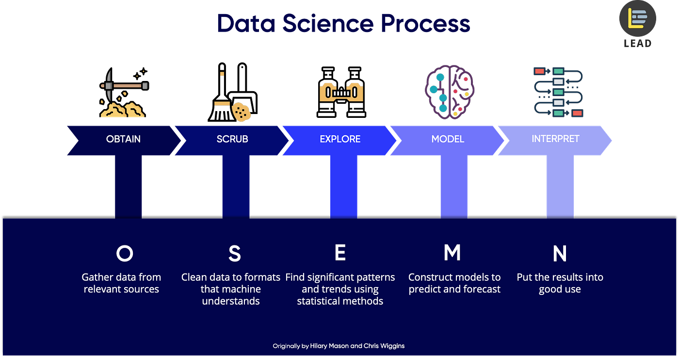
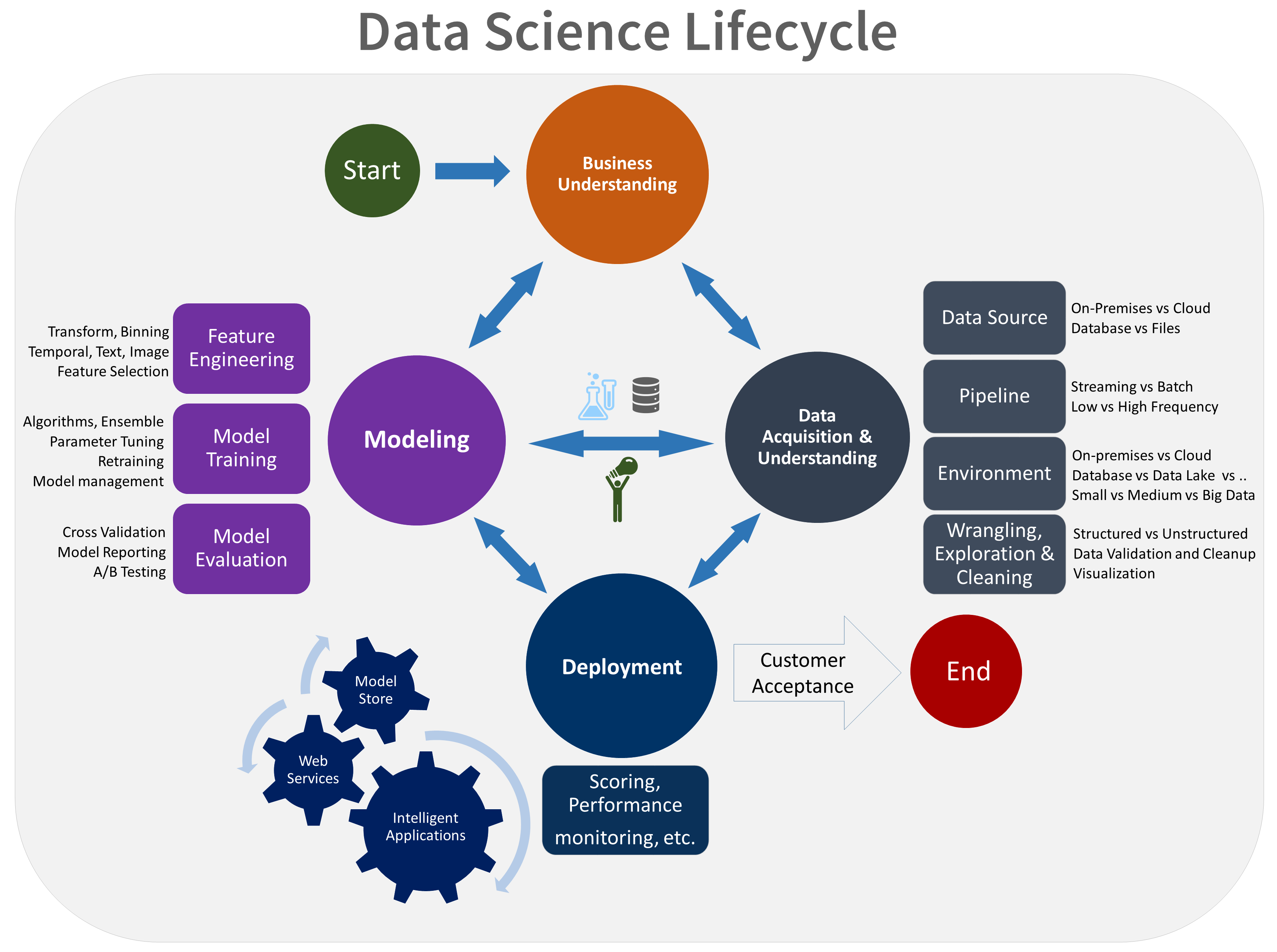
All references' style follow the APA7 format based on UoM APA7 Guide.

Repositories

MLfromscratch, https://github.com/python-engineer/MLfromscratch/.
Azure-TDSP-ProjectTemplate, https://github.com/Azure/Azure-TDSP-ProjectTemplate.

Math Miscs

Wikipedia. (14, Jan 2022). Minkoski distance. https://en.wikipedia.org/wiki/Minkowski_distance.
Wikipedia. (21, Apr 2022). Probability theory. https://en.wikipedia.org/wiki/Probability_theory.
Wikipedia. (20, Feb 2022). Statistics. https://en.wikipedia.org/wiki/Statistics.
Wikipedia. (6, May 2022). Operational research. https://en.wikipedia.org/wiki/Operations_research.
Wikipedia. (21, May 2022). Voting. https://en.wikipedia.org/wiki/Voting#Voting_methods.
Elaine, J H & Jonathan, G. (11, Nov 2021). What is mathematics. https://www.livescience.com/38936-mathematics.html.

Machine Learning Articles

Onel, H. (11, Sep 2018). Machine Learning Basics with the K-Nearest Neighbors Algorithm. https://towardsdatascience.com/machine-learning-basics-with-the-k-nearest-neighbors-algorithm-6a6e71d01761)
Wikipedia. (26, May 2022). Machine learning. https://en.wikipedia.org/wiki/Machine_learning.

Artificial Intelligence Articles

Wikipedia. (30, May 2022). Artificial Intelligent. https://en.wikipedia.org/wiki/Artificial_intelligence.
Java T Point. (2022). Artificial Intelligent. https://www.javatpoint.com/artificial-intelligence-tutorial.
Geeks for Geeks. (26, Feb 2022). Difference between Informed and Uninformed Search in AI. https://www.geeksforgeeks.org/difference-between-informed-and-uninformed-search-in-ai/.
Wikipedia. (9, May 2022). Monte Carlo Tree Search. https://en.wikipedia.org/wiki/Monte_Carlo_tree_search.
Sagar, S. (1, Aug, 2018). Monte Carlo Tree Search, MCTS For Every Data Science Enthusiast. https://towardsdatascience.com/monte-carlo-tree-search-158a917a8baa.
Wikipedia. (10, May 2022). Temporal difference learning. https://en.wikipedia.org/wiki/Temporal_difference_learning.
Fisher, R., Perkins, S., Walker, A & Wolfar, E. Skeletonization/Medial Axis Transform. https://homepages.inf.ed.ac.uk/rbf/HIPR2/skeleton.html.
Wikipedia. (21, May 2022). Constraint Satisfaction Problem. https://en.wikipedia.org/wiki/Constraint_satisfaction_problem.
Nimmisha, S. (Dec 2022). Classification of stages of Diabetic Retinopathy using Deep Learning. https://www.researchgate.net/publication/347447352_Classification_of_stages_of_Diabetic_Retinopathy_using_Deep_Learning.

Data Structure

David, L & Sarah, L. (Mar, 2021). Data Structure. Search Data Management. https://www.techtarget.com/searchdatamanagement/definition/data-structure.
Java T Point. (2022). Linked list. https://www.javatpoint.com/ds-linked-list.

Others

GO FAIR. (2021). FAIR Principles*. https://www.go-fair.org/fair-principles/.
Isaac, S. (15, Apr 2022). What is CI/CD? Continuous integration and continuous delivery explained. https://www.infoworld.com/article/3271126/what-is-cicd-continuous-integration-and-continuous-delivery-explained.html.
Humanperf Software (3, May 2018). NowIUnderstand Glossary: the 5W1H method. https://www.humanperf.com/en/blog/nowiunderstand-glossary/articles/5W1H-method.
David, G. (16, May 2021). The 5W1H Method: Project management defined and applied. https://www.wimi-teamwork.com/blog/the-5w1h-method-project-management-defined-and-applied/.
Wikipedia. (7, May 2022). Scalability. https://en.wikipedia.org/wiki/Scalability.
CloudZero. (30, Jun 2021). Horizontal Vs. Vertical Scaling: How Do They Compare?. https://www.cloudzero.com/blog/horizontal-vs-vertical-scaling.
Kat, B. (26, Dec 2021). How to write SMART goals. https://www.atlassian.com/blog/productivity/how-to-write-smart-goals.
Geeks For Geeks. (24, Aug 2021). Class method vs Static method in Python. https://www.geeksforgeeks.org/class-method-vs-static-method-python/.
Cher, H L. (3, Jan 2019). 5 Steps of a Data Science Project Lifecycle. https://towardsdatascience.com/5-steps-of-a-data-science-project-lifecycle-26c50372b492.
Salesforce. (2021). CRM 101: What is CRM. https://www.salesforce.com/crm/what-is-crm/.
Wikipedia. (5, Apr 2022). Cross-industry standard process for data mining. https://en.wikipedia.org/wiki/Cross-industry_standard_process_for_data_mining.
Microsoft. (2022). What is the Team Data Science Process?. https://docs.microsoft.com/en-us/azure/architecture/data-science-process/overview.
Atlassian. (2022). Agile Coach. https://www.atlassian.com/agile.
Wrike. (2022). What Is Waterfall Project Management?. https://www.wrike.com/project-management-guide/faq/what-is-waterfall-project-management/.
APPDYNAMICS. (2022). What is Database Management Systems (DBMS)?. https://www.appdynamics.com/topics/database-management-systems.
Wikipedia. (16, May 2022). Dimensionality reduction. https://en.wikipedia.org/wiki/Dimensionality_reduction.
Zook, M., Barocas, S., Boyd, D., Crawford, K., Keller, E., Gangadharan, S. P., ... & Pasquale, F. (2017). Ten simple rules for responsible big data research. PLoS computational biology, 13(3), e1005399. https://journals.plos.org/ploscompbiol/article?id=10.1371/journal.pcbi.1005399.

@rNLKJA

eczww / uom-ds-2019-2024 Goto Github PK

uom-ds-2019-2024's Introduction