This repository contains the data and scripts that maintain and build the gmt-gshhg package used by GMT.
GMT uses the coast utility to access a version of the GSHHG data specially formatted for GMT. The GSHHG data have strengths and weaknesses. It is global and open source, but is based on relatively old datasets and hence may not be accurate enough for very large-scale mapping projects. The current GSHHG version used by GMT is 2.3.7. Below is a mostly technical description of how the GSHHG data set was assembled, processed, and formatted to meet the requirements of GMT.
You can download the latest gshhg-gmt package from GitHub releases or from the GMT main site.
We will demonstrate the power of this database by starting with a regional hemisphere map centered near Papua New Guinea and zoom in on a specified point. The map regions will be specified in projected km from the projection center, e.g., we may want the map to go from km to km in the longitudinal and the latitudinal direction. Also, as we zoom in on the projection center we want to draw the outline of the next map region on the plot. To do that we use the -SJ option in plot.
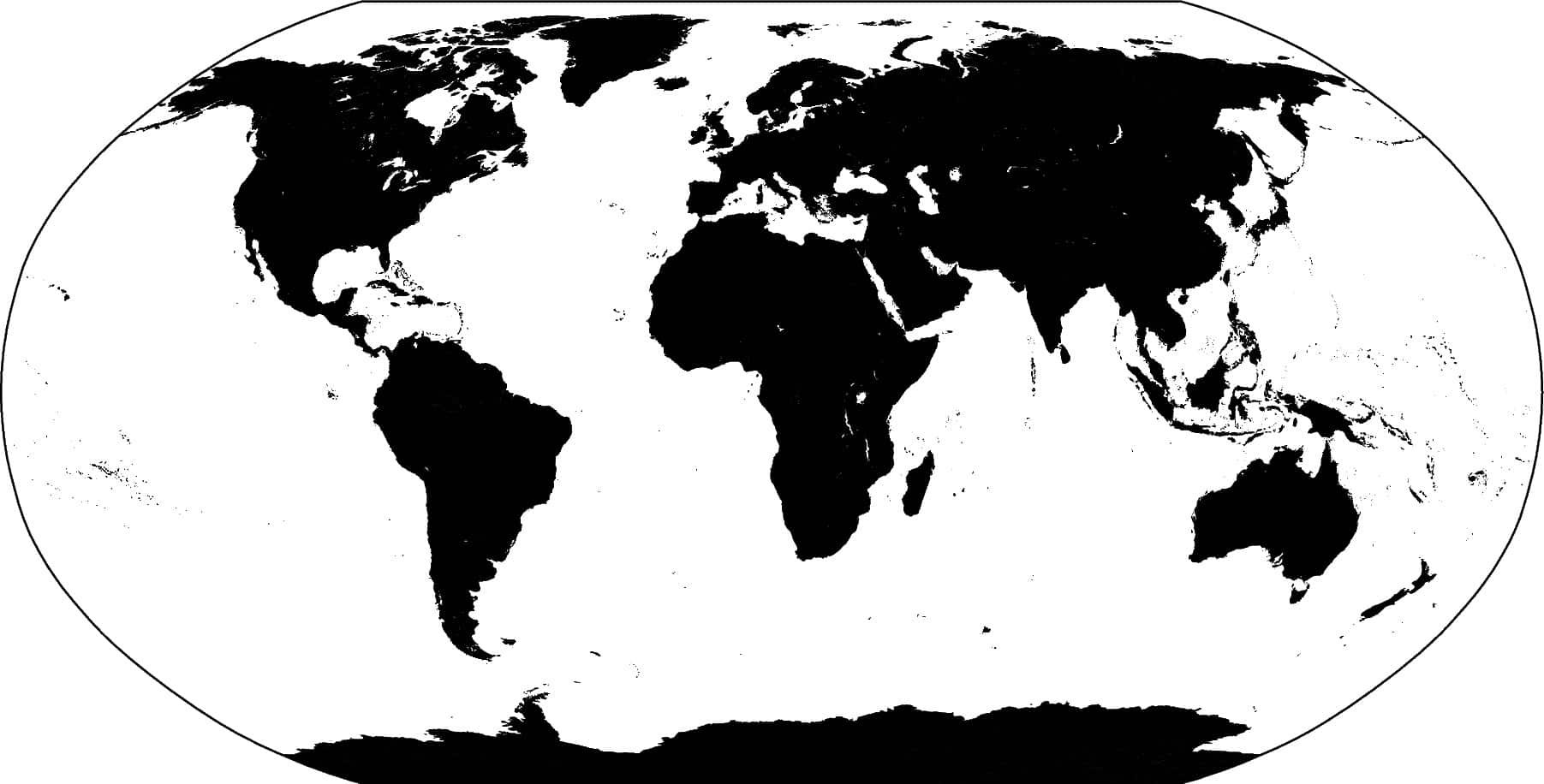
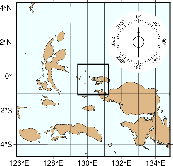
We begin with an azimuthal equidistant map of the hemisphere centered on 130°21'E, 0°12'S, which is slightly west of New Guinea, near the Strait of Dampier. The edges of the map are all 9000 km true distance from the projection center. At this scale (and for global maps) the crude resolution data will usually be adequate to capture the main geographic features. To avoid cluttering the map with insignificant detail we only plot features (i.e., polygons) that exceed 500 km2 in area. Smaller features would only occupy a few pixels on the plot and make the map look "dirty". We also add national borders to the plot. The crude database is heavily decimated and simplified by the DP-routine: The total file size of the coastlines, rivers, and borders database is only 283 kbytes. The plot is produced by the script:
gmt begin GMT_App_K_1
    gmt set GMT_THEME cookbook
    gmt set MAP_GRID_CROSS_SIZE_PRIMARY 0  MAP_ANNOT_MIN_SPACING 0.3i \
        MAP_ANNOT_OBLIQUE lon_parallel,lat_horizontal,tick_normal
    gmt coast -R-9000/9000/-9000/9000+uk -JE130.35/-0.2/3.5i -Dc \
	    -A500 -Gburlywood -Sazure -Wthinnest -N1/thinnest,- -B20g20 -BWSne
    echo 130.35 -0.2 | gmt plot -SJ-4000 -Wthicker
gmt end show
Here, we use the MAP_ANNOT_OBLIQUE setting to achieve horizontal annotations and set MAP_ANNOT_MIN_SPACING to suppress some longitudinal annotations near the S pole that otherwise would overprint. The square box indicates the outline of the next map.
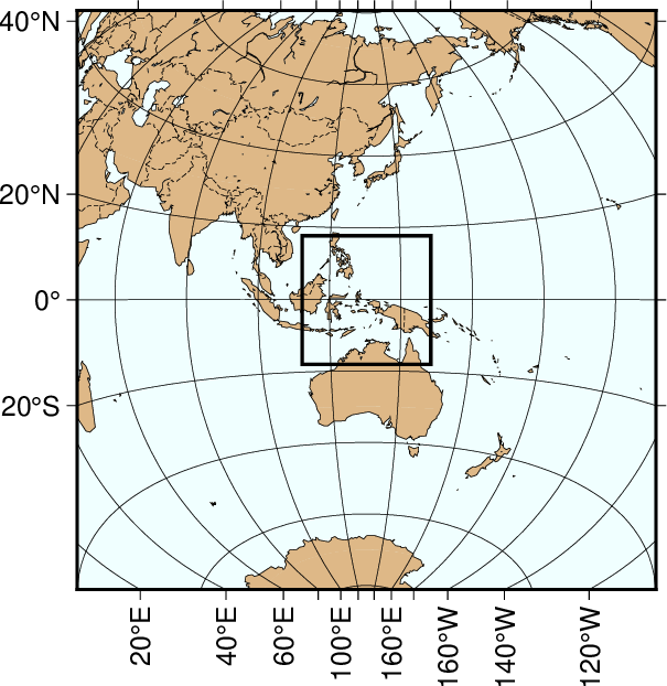
We have now reduced the map area by zooming in on the map center. Now, the edges of the map are all 2000 km true distance from the projection center. At this scale we choose the low resolution data that faithfully reproduce the dominant geographic features in the region. We cut back on minor features less than 100 km2 in area. We still add national borders to the plot. The low database is less decimated and simplified by the DP-routine: The total file size of the coastlines, rivers, and borders combined grows to 907 kbytes; it is the default resolution in GMT. The plot is generated by the script:
gmt begin GMT_App_K_2
    gmt set GMT_THEME cookbook
    gmt coast -R-2000/2000/-2000/2000+uk -JE130.35/-0.2/3.5i -Dl -A100 \
	    -Gburlywood -Sazure -Wthinnest -N1/thinnest,- -B10g5 -BWSne
    echo 130.35 -0.2 | gmt plot -SJ-1000 -Wthicker
gmt end show
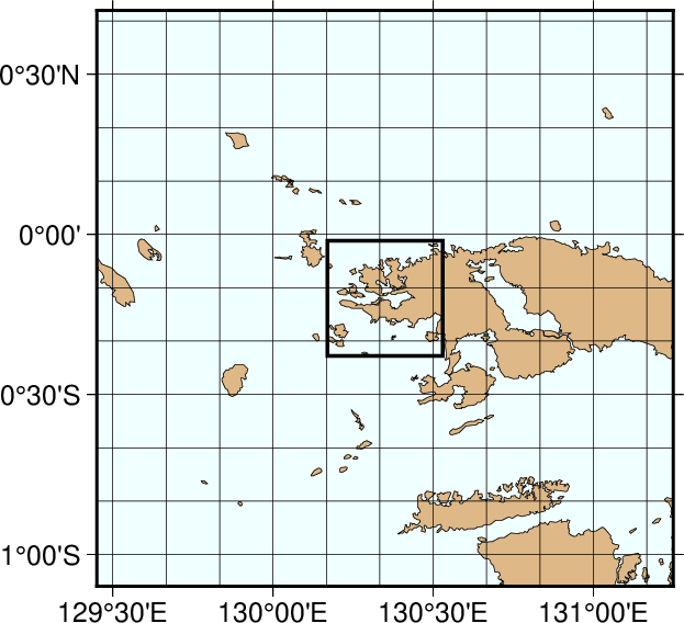
We continue to zoom in on the map center. In this map, the edges of the map are all 500 km true distance from the projection center. We abandon the low resolution data set as it would look too jagged at this scale and instead employ the intermediate resolution data that faithfully reproduce the dominant geographic features in the region. This time, we ignore features less than 20 km2 in area. Although the script still asks for national borders none exist within our region. The intermediate database is moderately decimated and simplified by the DP-routine: The combined file size of the coastlines, rivers, and borders now exceeds 3.35 Mbytes. The plot is generated by the script:
gmt begin GMT_App_K_3
    gmt set GMT_THEME cookbook
    gmt coast -R-500/500/-500/500+uk -JE130.35/-0.2/3.5i -Di -A20 -Gburlywood -Sazure -Wthinnest -N1/thinnest,- -B2g1 -BWSne
    echo 133 2 | gmt plot -Sc1.4i -Gwhite
    gmt basemap -Tmg133/2+w1i+t45/10/5+jCM --FONT_TITLE=12p --MAP_TICK_LENGTH_PRIMARY=0.05i --FONT_ANNOT_SECONDARY=8p
    echo 130.35 -0.2 | gmt plot -SJ-200 -Wthicker
gmt end show
The relentless zooming continues! Now, the edges of the map are all 100 km true distance from the projection center. We step up to the high resolution data set as it is needed to accurately portray the detailed geographic features within the region. Because of the small scale we only ignore features less than 1 km2 in area. The high resolution database has undergone minor decimation and simplification by the DP-routine: The combined file size of the coastlines, rivers, and borders now swells to 12.3 Mbytes. The map and the final outline box are generated by these commands:
gmt begin GMT_App_K_4
    gmt set GMT_THEME cookbook
    gmt coast -R-100/100/-100/100+uk -JE130.35/-0.2/3.5i -Dh -A1 \
	    -Gburlywood -Sazure -Wthinnest -N1/thinnest,- -B30mg10m -BWSne
    echo 130.35 -0.2 | gmt plot -SJ-40 -Wthicker
gmt end show
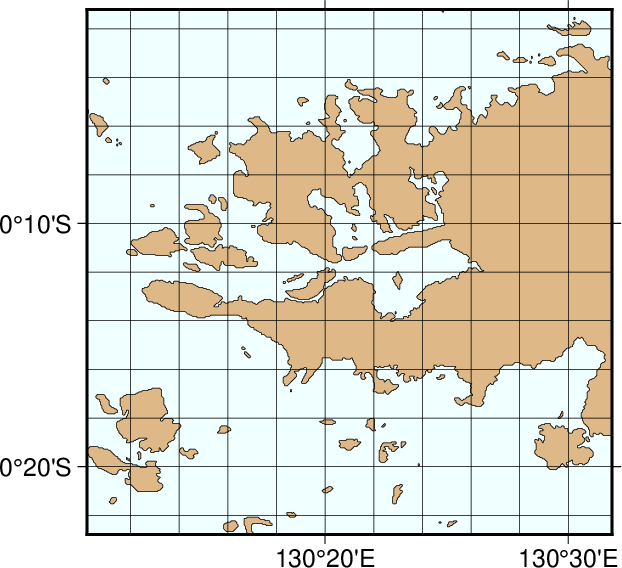
We now arrive at our final plot, which shows a detailed view of the western side of the small island of Waigeo. The map area is approximately 40 by 40 km. We call upon the full resolution data set to portray the richness of geographic detail within this region; no features are ignored. The full resolution has undergone no decimation and it shows: The combined file size of the coastlines, rivers, and borders totals a (once considered hefty) 55.9 Mbytes. Our final map is reproduced by the single command:
gmt begin GMT_App_K_5
    gmt set GMT_THEME cookbook
    gmt coast -R-20/20/-20/20+uk -JE130.35/-0.2/3.5i -Df -Gburlywood -Sazure -Wthinnest -N1/thinnest,- -B10mg2m -BWSne
gmt end show
We hope you will study these examples to enable you to make efficient and wise use of this vast data set.
There are two well-known public-domain data sets that could be used for this purpose. Once is known as the World Data Bank II or CIA Data Bank (WDB) and contains coastlines, lakes, political boundaries, and rivers. The other, the World Vector Shoreline (WVS) only contains shorelines between saltwater and land (i.e., no lakes). It turns out that the WVS data is far superior to the WDB data as far as data quality goes, but as noted it lacks lakes, not to mention rivers and borders. We decided to use the WVS whenever possible and supplement it with WDB data. We got these data over the Internet; they are also available on CD-ROM from the National Centers for Environmental Information, Boulder, Colorado.
In order to paint continents or oceans it is necessary that the coastline data be organized in polygons that may be filled. Simple line segments can be used to draw the coastline, but for painting polygons are required. Both the WVS and WDB data consists of unsorted line segments: there is no information included that tells you which segments belong to the same polygon (e.g., Australia should be one large polygon). In addition, polygons enclosing land must be differentiated from polygons enclosing lakes since they will need different paint. Finally, we want coast to be flexible enough that it can paint the land or the oceans or both. If just land (or oceans) is selected we do not want to paint those areas that are not land (or oceans) since previous plot programs may have drawn in those areas. Thus, we will need to combine polygons into new polygons that lend themselves to fill land (or oceans) only (Note that older versions of coast always painted lakes and wiped out whatever was plotted beneath).
The WVS and WDB together represent more than 100 Mb of binary data and something like 20 million data points. Hence, it becomes obvious that any manipulation of these data must be automated. For instance, the reasonable requirement that no coastline should cross another coastline becomes a complicated processing step.
-
To begin, we first made sure that all data were "clean", i.e., that there were no outliers and bad points. We had to write several programs to ensure data consistency and remove "spikes" and bad points from the raw data. Also, crossing segments were automatically "trimmed" provided only a few points had to be deleted. A few hundred more complicated cases had to be examined semi-manually.
-
Programs were written to examine all the loose segments and determine which segments should be joined to produce polygons. Because not all segments joined exactly (there were non-zero gaps between some segments) we had to find all possible combinations and choose the simplest combinations. The WVS segments joined to produce more than 200,000 polygons, the largest being the Africa-Eurasia polygon which has 1.4 million points. The WDB data resulted in a smaller data base (~25% of WVS).
-
We now needed to combine the WVS and WDB data bases. The main problem here is that we have duplicates of polygons: most of the features in WVS are also in WDB. However, because the resolution of the data differ it is nontrivial to figure out which polygons in WDB to include and which ones to ignore. We used two techniques to address this problem. First, we looked for crossovers between all possible pairs of polygons. Because of the crossover processing in step 1 above we know that there are no remaining crossovers within WVS and WDB; thus any crossovers would be between WVS and WDB polygons. Crossovers could mean two things: (1) A slightly misplaced WDB polygon crosses a more accurate WVS polygon, both representing the same geographic feature, or (2) a misplaced WDB polygon (e.g., a small coastal lake) crosses the accurate WVS shoreline. We distinguished between these cases by comparing the area and centroid of the two polygons. In almost all cases it was obvious when we had duplicates; a few cases had to be checked manually. Second, on many occasions the WDB duplicate polygon did not cross its WVS counterpart but was either entirely inside or outside the WVS polygon. In those cases we relied on the area-centroid tests.
-
While the largest polygons were easy to identify by visual inspection, the majority remain unidentified. Since it is important to know whether a polygon is a continent or a small pond inside an island inside a lake we wrote programs that would determine the hierarchical level of each polygon. Here, level = 1 represents ocean/land boundaries, 2 is land/lakes borders, 3 is lakes/islands-in-lakes, and 4 is islands-in-lakes/ponds-in-islands-in-lakes. Level 4 was the highest level encountered in the data. To automatically determine the hierarchical levels we wrote programs that would compare all possible pairs of polygons and find how many polygons a given polygon was inside. Because of the size and number of the polygons such programs would typically run for 3 days on a Sparc-2 workstation.
-
Once we know what type a polygon is we can enforce a common "orientation" for all polygons. We arranged them so that when you move along a polygon from beginning to end, your left hand is pointing toward "land". At this step we also computed the area of all polygons since we would like the option to plot only features that are bigger than a minimum area to be specified by the user.
-
Obviously, if you need to make a map of Denmark then you do not want to read the entire 1.4 million points making up the Africa-Eurasia polygon. Furthermore, most plotting devices will not let you paint and fill a polygon of that size due to memory restrictions. Hence, we need to partition the polygons so that smaller subsets can be accessed rapidly. Likewise, if you want to plot a world map on a letter-size paper there is no need to plot 10 million data points as most of them will plot several times on the same pixel and the operation would take a very long time to complete. We chose to make 5 versions on the database, corresponding to different resolutions. The decimation was carried out using the Douglas-Peucker (DP) line-reduction algorithm (Douglas and Peucker, 1973). We chose the cutoffs so that each subset was approximately 20% the size of the next higher resolution. The five resolutions are called full, high, intermediate, low, and crude; they are accessed in coast, gmtselect, and grdlandmask with the -D option. For each of these 5 data sets (f, h, i, l, c) we specified an equidistant grid (1, 2, 5, 10, 20) and split all polygons into line-segments that each fit inside one of the many boxes defined by these grid lines. Thus, to paint the entire continent of Australia we instead paint many smaller polygons made up of these line segments and gridlines. Some book-keeping has to be done since we need to know which parent polygon these smaller pieces came from in order to prescribe the correct paint or ignore if the feature is smaller than the cutoff specified by the user. The resulting segment coordinates were then scaled to fit in short integer format to preserve precision and written in netCDF format for ultimate portability across hardware platforms (Wessel and Smith, 1996).
-
While we are now back to a file of line-segments we are in a much better position to create smaller polygons for painting. Two problems must be overcome to correctly paint an area:
-
We must be able to join line segments and grid cell borders into meaningful polygons; how we do this will depend on whether we want to paint the land or the oceans.
-
We want to nest the polygons so that no paint falls on areas that are "wet" (or "dry"); e.g., if a grid cell completely on land contains a lake with a small island, we do not want to paint the lake and then draw the island, but paint the annulus or "donut" that is represented by the land and lake, and then plot the island.
GMT uses a polygon-assembly routine that carries out these tasks on the fly.
-
- Bohlander, J. and T. Scambos. 2007. Antarctic coastlines and grounding line derived from MODIS Mosaic of Antarctica (MOA), Boulder, Colorado USA: National Snow and Ice Data Center.
- Douglas, D.H., and T. K. Peucker, 1973, Algorithms for the reduction of the number of points required to represent a digitized line or its caricature, Canadian Cartographer, 10, 112–122.
- Gorny, A. J. (1977), World Data Bank II General User GuideRep. PB 271869, 10pp, Central Intelligence Agency, Washington, DC.
- Soluri, E. A., and V. A. Woodson (1990), World Vector Shoreline, Int. Hydrograph. Rev., LXVII(1), 27–35.
- Wessel, P., and W. H. F. Smith (1996), A global, self-consistent, hierarchical, high-resolution shoreline database, J. Geophys. Res., 101(B4), 8741–8743.
- Paul Wessel Primary contact: [email protected]
- Walter H. F. Smith
The detailed changelog is available here.
The project is distributed under the GNU Lesser General Public License.
Version 2.3.7 June 15, 2017
Updates the Northern Mariana Islands with CUPS data from NOAA, adds two missing islands to northern Norway, and adds in the missing Kosovo-Serbia boundary.
Version 2.3.6 August 19, 2016
Fixed 11 crossings in Antarctica grounding line and one in the ice front. Added missing islands Georgetown and MacMahan, ME, and updated Jan Mayen, Norway [thanks to Norwegian Polar Institute]
Version 2.3.5 April 12, 2016
Added missing boundary between Sudan and South Sudan. Fixed non-closure of the Slovenia, Croatia and Hungary borders.
Version 2.3.4 Jan 1, 2015
Corrected formatting error in the binary versions of the borders and rivers files. Added "Lake" Maelaren (Sweden) to the coastline which reverted 11 "lakes" to their proper status as islands.
Version 2.3.3 Nov 2014:
Removed the obsolete Saudi-Kuwait Neutral Zone diamond-shaped border and replaced with something resembling what Google Earth shows.
Version 2.3.2 August 2014:
Removed several internal crossovers for the two new Antarctica polygons. All other polygons are unchanged.
Version 2.3.1 July 2014:
Updated to include Peter I Island near Antarctica which had gone missing during the switch to the Antarctica data source for 2.3.0.
Version 2.3.0 Feb 2014:
This data set consists of three related components:
GSHHS: Global Self-consistent Hierarchical High-resolution Shorelines: These originate as individual polygons at five different resolutions. The ocean-land shorelines derive from WVS (World Vector Shoreline project) [Soluri and Woodson, 1990] while the polygons for lakes, islands-in-lakes, and ponds-in-islands- in-lakes derive from WDBII [Gorny, 1977], which is a much older and lower-quality data product. Our compilation combines these data into a self-consistent product; see Wessel and Smith [1996] for processing details. Over the years we have manually added new data in areas that were poorly represented in the original data set; however, as users zoom in closely they can see that the old data may in places be mis-registered relative to recent data such as used in Google Earth. AC: Starting with release 2.3.0 we have replaced the poor Antarctica polygon and associated islands with newer and more accurate data from Bohlander and Scambos (2007) via Atlas of the Cryosphere. This lets us consider two polygon: ice-line and grounding line. New processing was needed to allow a run-time switch on which polygon to use (since it changes how many islands to include). Antarctic ice-front polygons are given level 5 while Antarctic grounding-line polygons are given level 6. Non-GMT users of these data should skip one of these two levels are reset the other one to level = 1. The next GMT5 release 5.2.0 will allow users to select their Antarctica coastline while older versions will simply use the ice-front line as the single Antarctica coastline; the grounding line data are not visible to those versions.
WDBII: CIA World Data Bank II lineaments for borders and rivers. Over the years, political boundaries have changed and we have updated these to reflect realities based on feedback from our users. As mentioned above, WDBII is also used for lakes.
GSHHG is distributed in several representations:
1. The binary and shapefile distributions provide the complete
   GSHHS polygons and WDBII lineaments in their five resolutions
   (i.e., after our full processing), and differ only in the
   file formats (native binary data files versus standard GIS
   shapefiles).  These distributions are normally used by
   users interested to use these data outside the standard
   GMT-based environment, or GMT users who wish to access the
   whole GSHHS polygons.
2. The netCDF distribution provides specially processed netCDF
   representations of GSHHS and WDBII where the polygons and
   lines have been subdivided and indexed to deliver rapid map-
   making for GMT.  Users who wish to access GSHHG outside of
   GMT are advised to use the binary and shapefile version of
   the actual polygons as there is no user documentation for
   how to access the netCDF files.
Many thanks to Tom Kratzke, Metron Inc., for patiently testing many draft versions of GSHHS and reporting inconsistencies such as erratic data points and crossings.
Version 2.2.4 Nov 2013: We added three missing lakes (Mono, Trinity, and Isabella) in California, plus two islands in Lake Mono. Also found a bug in polygon_consistency that failed to find some spikes (~20-25 polygons affected), as well as an incorrect lake in Antarctica.
Version 2.2.3 July 2013: We eliminated ~120 spikes (< 2m thick excursions) from a few dozen full resolution polygons. Also fixed an old mistake in Baffin Island in all but the crude resolution; this also converted two mislabeled "lakes" into islands in the full and high resolution data.
Version 2.2.2 January 2013: We have removed Sandy Island, Coral Sea (non feature), shifted Society Island polygons ~1 arc minute to the west, and replaced Mehetia Island with better data. Furthermore, 50 islands that were imprecise duplicates of more accurate WVS features were removed. Apart from the Agalega islands, these duplicates were mostly found in the Red Sea, the Persian Gulf, and in the Cook-Austral region. GSHHG is now released under the lesser GNU License, v3 or any earlier version.
Version 2.2.1 July 2012: We have renamed the product GSHHG since it contains more than just shorelines (we distribute political boundaries and rivers as well). The GSHHG building and distribution is now fully decoupled from GMT. We have also changed the name of the netCDF files for GMT to use the more standard extension *.nc. Furthermore, the packages have been renamed for clarity and follow the form gshhg-{gmt,bin,shp}-.{tar,zip} There are no significant changes to the actual data features, other than a glitch in SA-NT border in Australia and removal of 7 zero-length border segments. Following the rebranding to GSHHG the names of the distribution files have changed as well.
Version 2.2.0 July 2011: The area of small (< 0.1 km^2) polygons got truncated to 0. This would cause gshhs to consider them as lines (borders or rivers) instead of polygons. Furthermore, the areas were recomputed using the WGS-84 ellipsoid as the previous area values were based on a spherical calculation. Thanks to José Luis García Pallero for pointing this out. We now store the area with a magnitude scale tuned to each polygon. Also, the greenwich flag is now a 2-bit flag composed of 1 (crosses Greenwich), 2 (crosses Dateline), 3 (both) or 0 (no such crossing). See gshhs.[ch] for details. Finally, the binary gshhs files now store Antarctica in -180/+180 range so as to avoid a jump when dumped to ASCII. Also, the WDBII shapefiles only had the first 3 levels of rivers; version 2.2.0 has all 11. Finally, to be able to detect the river-lake features in the WDBII binary files we set the river flag to 1 if a closed feature.
Version 2.1.1 March 2011: Relatively minor fixes to low-resolution polygons, including editing errors introduced in v 2.1, removing a few spikes from 4-5 polygons, and fixing Germany-Poland border near the Baltic Sea.
Version 2.1 July 2010: Fixes lack of river-lake flag in the binary and shapefile release. Shapefile polygons of level = 2 and with a negative area are river-lakes. Also include WDBII border and river data as shapefiles.
version 2.0 July 15, 2009: Differs from the previous version 1.x in the following ways.
- Free from internal and external crossings and erratic spikes at all five resolutions.
- The original Eurasiafrica polygon has been split into Eurasia (polygon # 0) and Africa (polygon # 1) along the Suez canal.
- The original Americas polygon has now been split into North America (polygon # 2) and South America (polygon # 3) along the Panama canal.
- Antarctica is now polygon # 4 and Australia is polygon # 5, in all the five resolutions.
- Fixed numerous problems, including missing islands and lakes in the Amazon and Nile deltas.
- Flagged "riverlakes" which are the fat part of major rivers so they may easily be identified by users.
- Determined container ID for all polygons (== -1 for level 1 polygons) which is the ID of the polygon that contains a smaller polygon.
- Determined full-resolution ancestor ID for lower res polygons, i.e., the ID of the polygon that was reduced to yield the lower- res version.
- Ensured consistency across resolutions (i.e., a feature that is an island at full resolution should not become a lake in low!).
- Sorted tables on level, then on the area of each feature.
- Made sure no feature is missing in one resolution but present in the next lower resolution.
- Store both the actual area of the lower-res polygons and the area of the full-resolution ancestor so users may exclude fea- tures that represent less that a fraction of the original full area.
There was some duplication and wrong levels assigned to maritime political boundaries in the Persian Gulf that has been fixed.
These changes required us to enhance the GSHHG C-structure used to read and write the data. As of version 2.0 the header structure is
struct GSHHG {  /* Global Self-consistent Hierarchical High-resolution Shorelines */
        int id;         /* Unique polygon id number, starting at 0 */
        int n;          /* Number of points in this polygon */
        int flag;       /* = level + version << 8 + greenwich << 16 + source << 24 + river << 25 */
        /* flag contains 5 items, as follows:
         * low byte:    level = flag & 255: Values: 1 land, 2 lake, 3 island_in_lake, 4 pond_in_island_in_lake
         * 2nd byte:    version = (flag >> 8) & 255: Values: Should be 12 for GSHHG release 12 (i.e., version 2.2)
         * 3rd byte:    greenwich = (flag >> 16) & 1: Values: Greenwich is 1 if Greenwich is crossed
         * 4th byte:    source = (flag >> 24) & 1: Values: 0 = CIA WDBII, 1 = WVS
         * 4th byte:    river = (flag >> 25) & 1: Values: 0 = not set, 1 = river-lake and level = 2
         */
        int west, east, south, north;   /* min/max extent in micro-degrees */
        int area;       /* Area of polygon in 1/10 km^2 */
        int area_full;  /* Area of original full-resolution polygon in 1/10 km^2 */
        int container;  /* Id of container polygon that encloses this polygon (-1 if none) */
        int ancestor;   /* Id of ancestor polygon in the full resolution set that was the source of this polygon (-1 if none) */
};
Following each header structure is n structures of coordinates:
struct GSHHG_POINT {	/* Each lon, lat pair is stored in micro-degrees in 4-byte signed integer format */
	int32_t x;
	int32_t y;
};
Some useful information:
A) To avoid headaches the binary files were written to be big-endian. If you use the GMT supplement gshhg it will check for endian-ness and if needed will byte swab the data automatically. If not then you will need to deal with this yourself.
B) In addition to GSHHS we also distribute the files with political boundaries and river lines. These derive from the WDBII data set.
C) As to the best of our knowledge, the GSHHG data are geodetic longitude, latitude locations on the WGS-84 ellipsoid. This is certainly true of the WVS data (the coastlines). Lakes, riverlakes (and river lines and political borders) came from the WDBII data set which may have been on WGS072. The difference in ellipsoid is way less then the data uncertainties. Offsets have been noted between GSHHG and modern GPS positions.
D) Originally, the gshhs_dp tool was used on the full resolution data to produce the lower resolution versions. However, the Douglas-Peucker algorithm often produce polygons with self-intersections as well as create segments that intersect other polygons. These problems have been corrected in the GSHHG lower resolutions over the years. If you use gshhs_dp to generate your own lower-resolution data set you should expect these problems.
E) The shapefiles release was made by formatting the GSHHG data using the extended GMT/GIS metadata understood by OGR, then using ogr2ogr to build the shapefiles. Each resolution is stored in its own subdirectory (e.g., f, h, i, l, c) and each level (1-4) appears in its own shapefile. Thus, GSHHS_h_L3.shp contains islands in lakes for the high res data. Because of GIS limitations some polygons that straddle the Dateline (including Antarctica) have been split into two parts (east and west).
F) The netcdf-formatted coastlines distributed with GMT derives directly from GSHHG; however the polygons have been broken into segments within tiles. These files are not meant to be used by users other than via GMT tools (pscoast, grdlandmask, etc).