A 2019 project of mine revolved around some sophisticated ideas on how to implement neural networks. This work here is my first milestone to give it a face. I am proud to present custom connect, a new kind of neural network.
But watch out, the presentation is optimized for Full HD on a PC or laptop. Github dark mode should be used to get the real experience.
- Prolog
- Perceptron vs. Custom Perceptron
- Hyper Parameters
- Permutation of Neural Networks
- First Competitors
- First Competition
- The Custom Paradox
- Mixed Linearity
- Testing
- A good Layer Size
- Network Types in Comparison
- Efficiency
- New Net
- The last Layer should be Fully Connected
- Old vs. New
- Custom Pruning and Growing
- Ultra-Deep Net
- The Technique behind
- Issues Inside
- Uncomplexity
- Installation
- Summarized
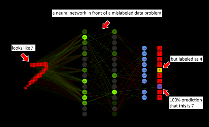
Fernanda Viégas from Google Brain talked in her lecture about how you can accelerate your machine learning skills by a factor of 10 by playing with data simulation and visualization tools. The best way to play is with a game. So why not take a neural network and turn it into a goodgame?
There are several ways to solve a problem with mislabeled data like in the example above. One technique that every machine learning (ML) engineer should know is to execute the forward pass and skip the backward pass and weight optimization when the prediction is more than 99%. It does not matter if the prediction was right or wrong. Nothing bad would happen in the example.
But the main reason is efficiency. To perform the forward pass, all weights must be used once. This calculation must be done to get a prediction. For the backward pass, the weight and delta arrays with the same length have to be executed again. The weight optimization step would also use all weights and deltas. Forward pass + backward pass + optimization ≈ 5 * forward pass. Good networks predict over 50% of the samples with a softmax probability over 99% after 60,000 MNIST training images, skipping these samples can save a large amount of computation. Suppose we have target = 1 and prediction = 1, target - prediction = error = 0, what to do? Do not calculate!
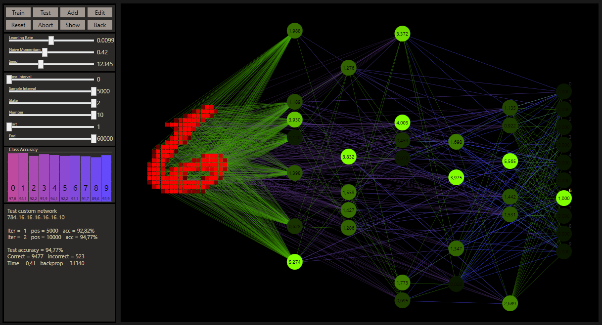
Note that ReLU was used as activation function for the hidden neurons. If the value is more than zero the value is taken, else the activation is set to zero. To simplify the visualization and focus on the important parts, zero nodes are no longer shown. The output neurons are activated with softmax. The batch size depends on the prediction, that means the weight update is executed only if the prediction was wrong. This idea was also used in the Mark I perceptron machine by Frank Rosenblatt. The same Glorot-uniform weight initialization is used for all tested networks.
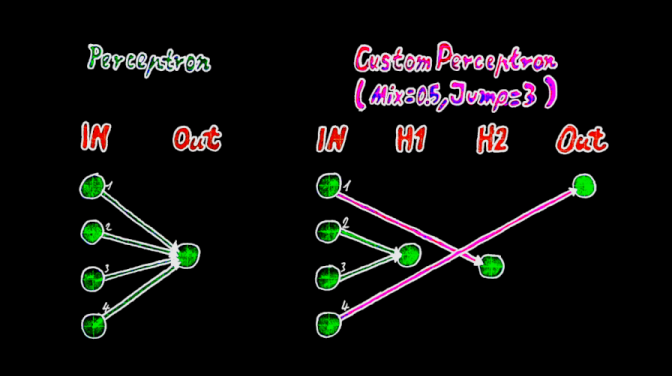
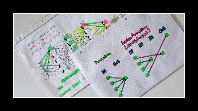
A neural network can be described as a collection of perceptrons. With many layers, this is also called a deep neural network (DNN) or a multi-layer perceptron (MLP). To understand custom connect, you need to know how a perceptron works. But instead of connecting the input neuron with its weight to the output neuron, the custom position is able to connect this input neuron with its weight to any neuron in the network. The weight position is the unique key to this.
Custom connect (cc) is simplified to three hyper parameters.
- Custom seed
- Custom mix
- Custom jump
The custom seed defines how the refixed connections connect randomly to the neurons, similiar to the weight seed to get random weight values. Before the positions can be set, the mix must first be selected. In addition, the custom seed in combination with the mix percentage randomly influences which weights are set and used as custom connections.
The custom mix sets the proportion of weights that are used as custom connections. A mix of 0% defines a deep neural network. A mix of 100% sets all weights as custom weights.
The custom jump sets the limit over how many layers the connections can randomly propagate. The minimum is 2, the maximum jump depends on the layer size and engaged the ability to connect every input neuron with every output neuron.

Equipped with the basics, let's suppose that 784 input neurons are active here, instead of 7 as in the animation, and think about what custom connect actually is. The default settings for this example are a network size of 784(in)-16(h1)-16(h2)-10(out), a mix = 0.5 and jump = 3. This network contains low connected a whole set of networks.
784(in)-16(h1)-16(h2)-10(out)784(in)-16(h1)-10(out)784(in)-16(h2)-10(out)784(in)-10(out)
If we consider the original 784-16-16-10 network with a jump of 2 instead of 3 and a mixing of 50% as before, this network can be remodeled into a sparsely connected 784-32-10 network. Where the h1 neurons pass their signals to the h2 neurons.
784(in)-32(h2 += h1)-10(out)
With the reinforced connections and especially with more layers, it gets really complicated to describe what it is. Another important point is that cc uses the same number of weights as the deep neural network. Moreover, it also uses the same weight values.
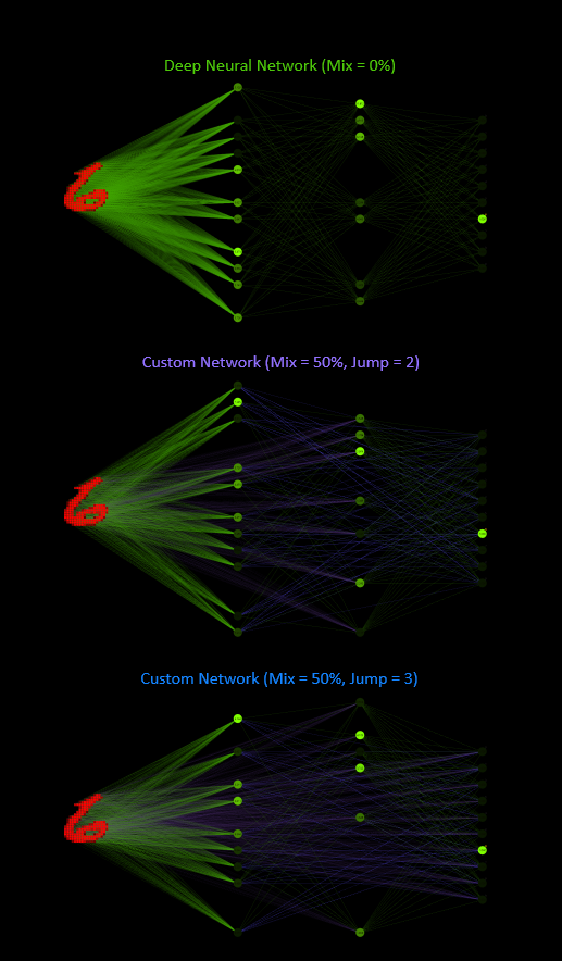
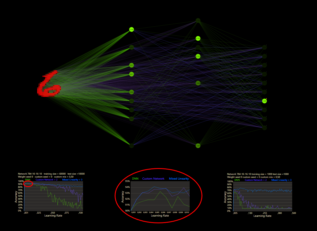
These are the networks for a first test. All three types are based on the same source, a 784-16-16-10 network with ReLU activation for the hidden neurons and softmax for the output neurons to get a final prediction. The respective font color represents the network shown in the upcoming tests.
This was my first impression old vs. new after the implementation was working. The designer helps to create the custom networks with the available hyper parameters.
| Training | Test | |
|---|---|---|
| DNN | 90.38% | 93.29% |
| CCJ2 | 91.44% | 93.66% |
| CCJ3 | 91.63% | 93.81% |
A good start!
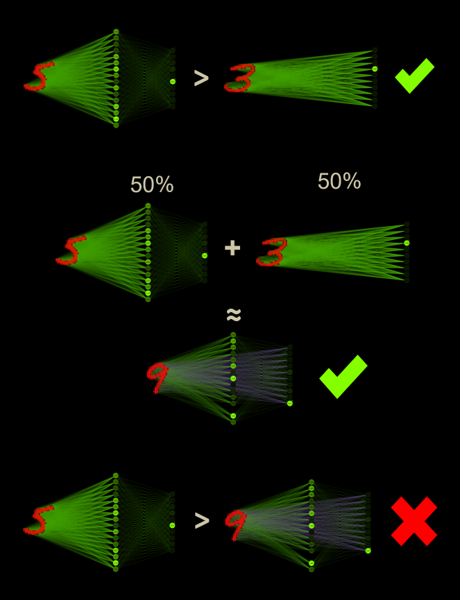
It is well known that neural networks are much more powerful than networks without hidden neurons. A neural network versus multiclass logistic regression. ML enthusiasts would clearly bet on the neural network, quite right! But what happens when the better network uses 50% (784 * 16) as logistic regression weights? Contrary to all my intuition, a custom network with logistic regression components seems to perform better than without. The higher density of connections in the direction of the outputs could be the reason. Perhaps it is not a paradox at all, but a logical consequence.
Did you notice the many active ReLU neurons in this example? This is no coincidence, low learning rates cause more activation, high learning rates cause the dying ReLU problem.
Mixed linearity appears to be special in some sense. As far as I know, this term does not actually exist. But mixed linearity describes quite well what happens here. The simplest form of a perceptron system is logistic regression. Here, each input is directly connected to the output neuron. This is a linear connection with the ability to separate linear. With neural networks, the idea of hidden neurons began. After input neurons are connected to a hidden neuron, they can behave non-linear. As it turns out, non-linearity is much more powerful for several reasons.
But when you compare the two approaches, you find some special abilities that make both types valuable. That's what cc takes advantage of, and perhaps more than expected. For example, logistic regression learns much faster and can't lose connectivity like ReLU-activated neurons. A layer of ReLU neurons, on the other hand, can make the network a better predictor and more efficient than logistic regression.
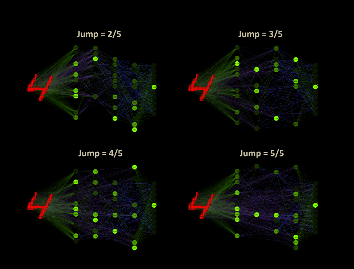
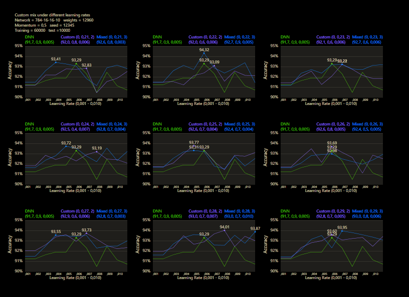
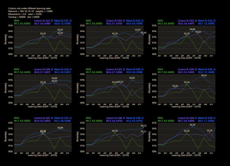
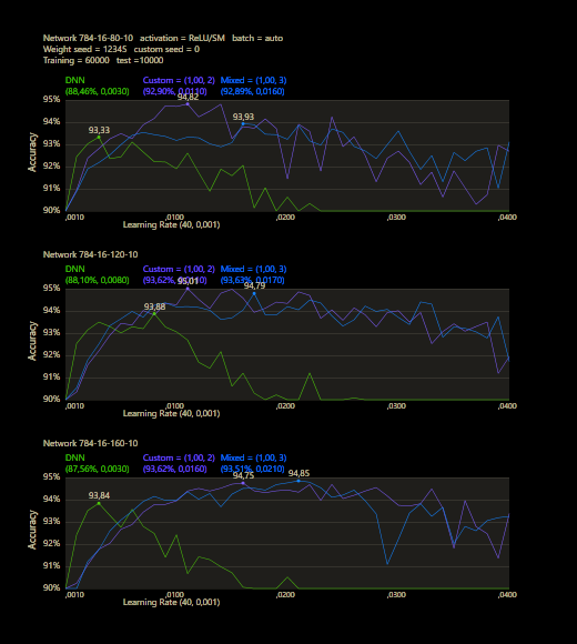
The training uses the entire MNIST dataset of 60,000 training images. Then the trained network is tested with 10,000 test images and the result is drawn. The reference network 784-16-16-10 achieved 93.29% in the test and was trained with a learning rate of 0.005 and a momentum rate of 0.5. This accuracy represents the benchmark reference. The momentum rate of 0.5 remains fixed in the next tests. Besides the hyper parameters, each network also contains (mean, std, best learning rate) for that graph.
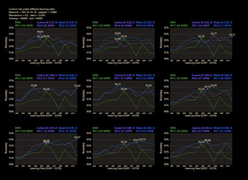
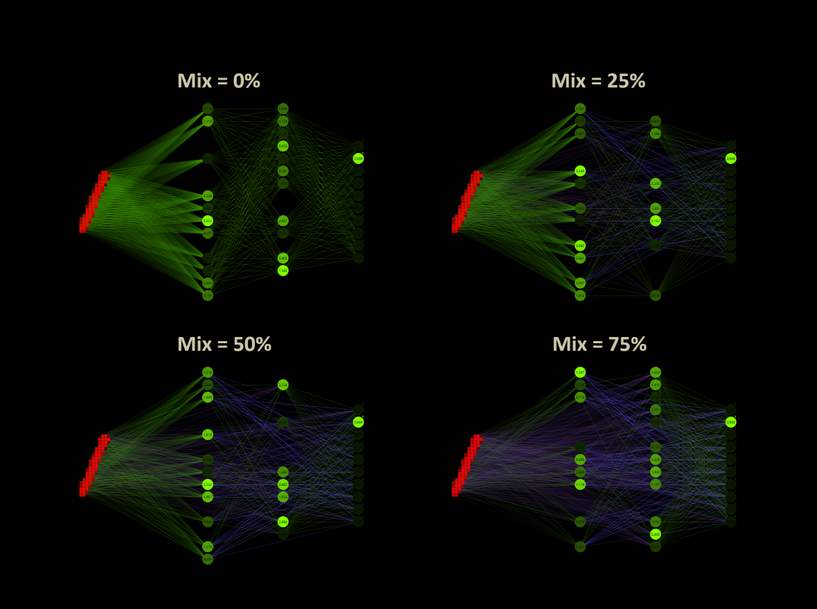
The prediction has already increased noticeably with a mix of only 10% and a jump of 2. At the other end with a mix of 90% and a jump of 3, the prediction has become strangely smooth. A mix between 40% and 60% close to the middle gave the highest results which were mostly above the DNN. I find it interesting that only the balance led to significantly better performance.
Mix 1 - 99
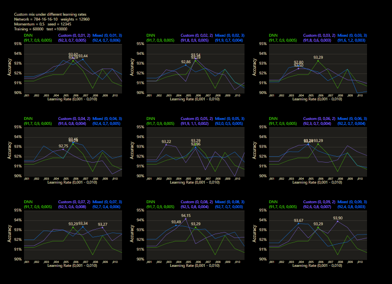
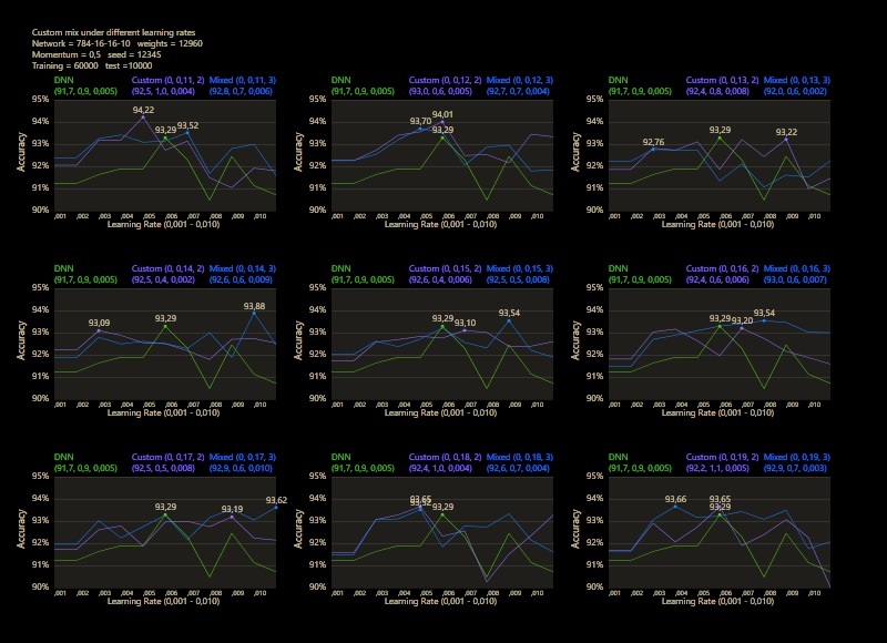
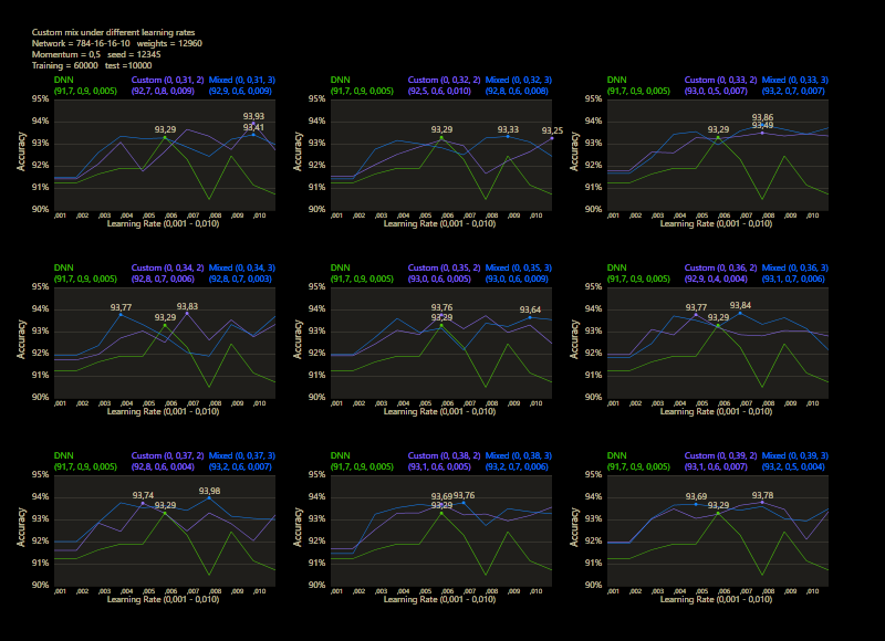
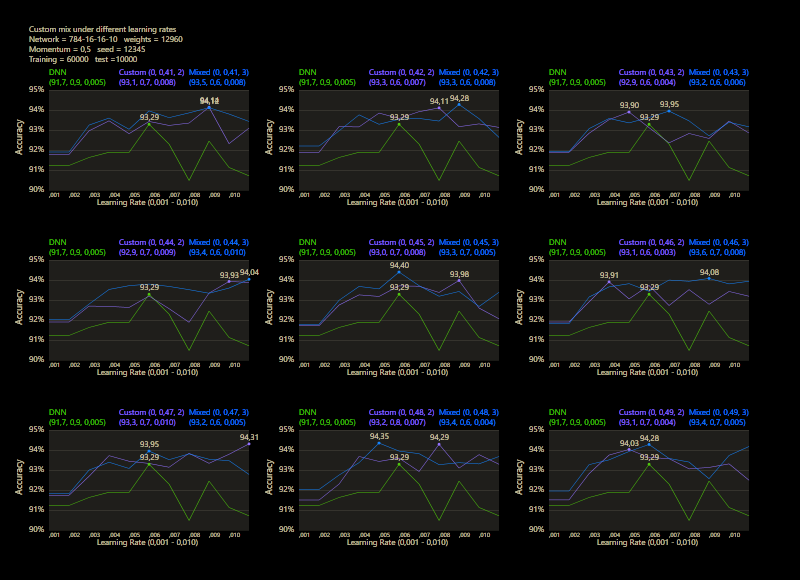

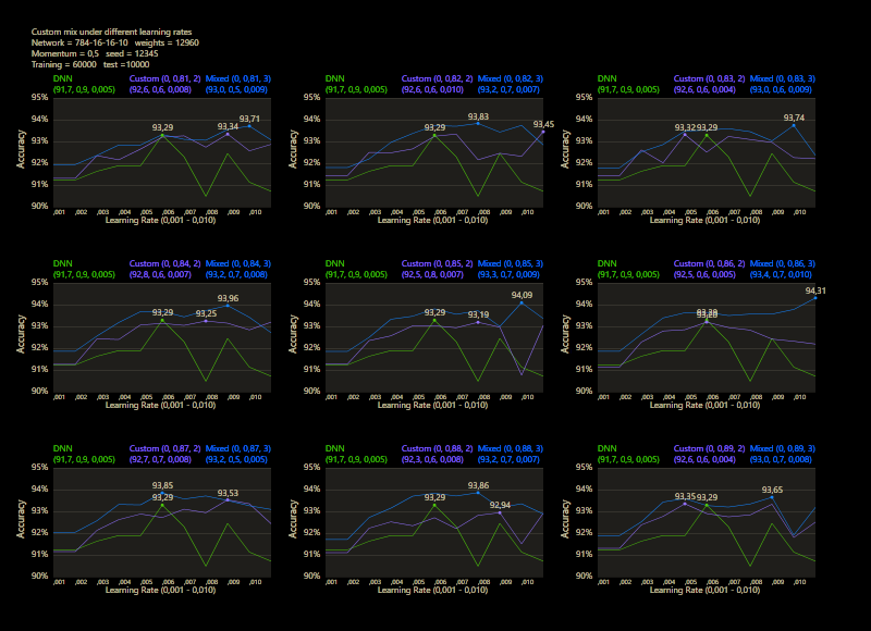
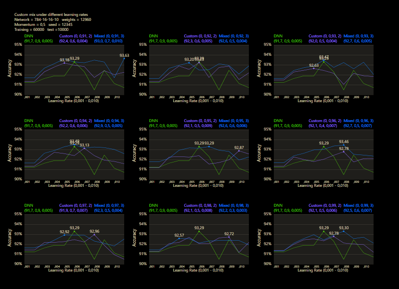
The test between 1% - 99% also shows that the learning rate should be set slightly higher with increasing mix. Noticeably, there were hardly any outliers that were worse than the DNN. The smoothness of the results was also impressive. With a new data set that requires its own parameters, it's relatively likely to make better predictions with cc, which should be closer to the peak values.
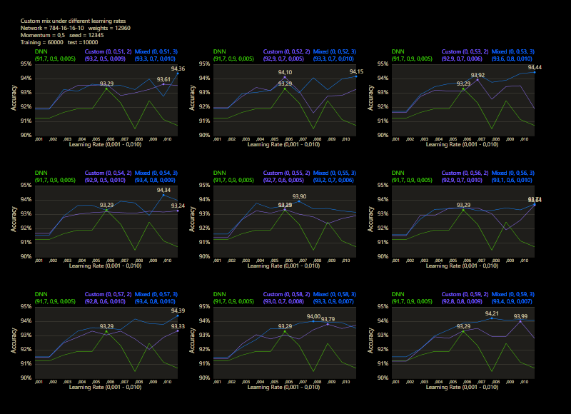
The best result with a jump of 2 gave an accuracy of 94.31% with a mix of 47% and a learning rate of 0.01.
A jump of 3 increased the accuracy to 94.52% with a mix of 66% and a learning rate of 0.008. A well-initialized DNN appears to be one of the subliminal advantages of cc, which may result in an even better predictor.
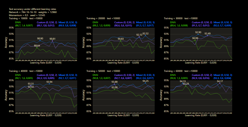
One of the major benefits can be observed under different training sizes, the custom connections accelerate learning. A jump of 3 dominated the DNN even under all conditions, no matter how many images were trained or what learning rate was used. Only 40,000 training images were required and cc was able to significantly outperform the DNN's prediction accuracy after training the entire training data set of 60,000 images.
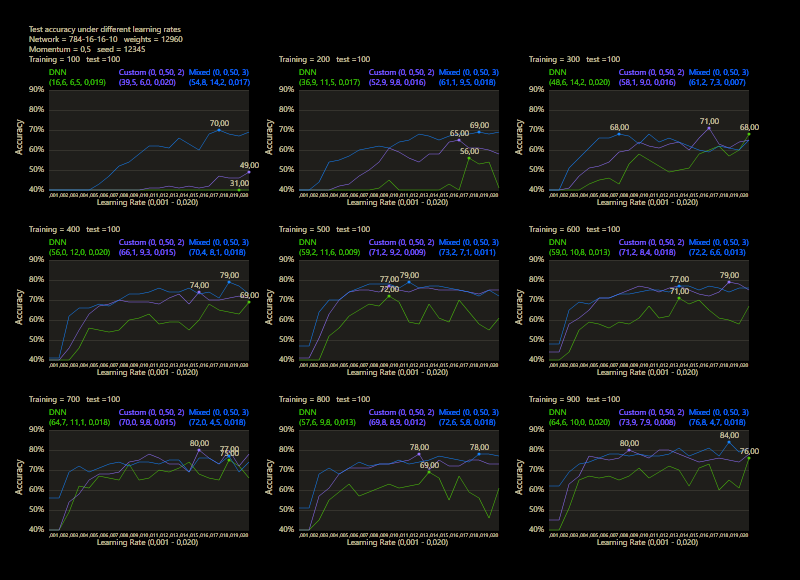
Mixed linearity works quite well under much smaller training data, 70% test accuracy after 100 training data is excellent.
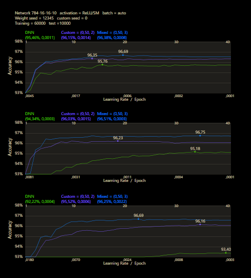
The training runs for each epoch through the entire MNIST dataset for 40 epochs. After each training epoch, the learning rate is multiplied by a factor of 0.9 and the momentum rate by a factor of 0.95.
Custom networks are shown to be very robust and work very reliably under different learning rates and can provide good results where DNNs are no longer stable.
The accuracy can be increased with more hidden neurons, quite simply.
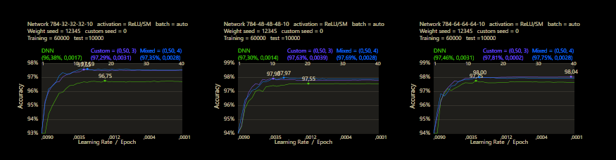
It was very impressive to see how quickly the limit of the MNIST dataset was reached with cc. However, it also becomes clear that the new method doesn't really work differently, only better. But the limit remains the same. Above an accuracy of 98% it hardly makes sense to use more neurons. Neural networks with more than 100 neurons on the first hidden layer seem oversized, cc networks reduce this around to 2/3 of the DNN size. If you want to break the 98% for MNIST significantly, you need other tricks like data augmentation and a convolutional network.
I was wondering how many layers should be used to get good predictions. With a little experimentation, this was the highest result with an accuracy of 94.77% with a network size of 784-16-16-16-16-16-10, a mix = 0.5 and jump = 5/6. All under the condition not to use more than 16 hidden neurons per layer. The layer size was much higher than a DNN would use, but with more layers it was easier to make better predictions. And also surprisingly, it was not a mixed linearity network that I found.
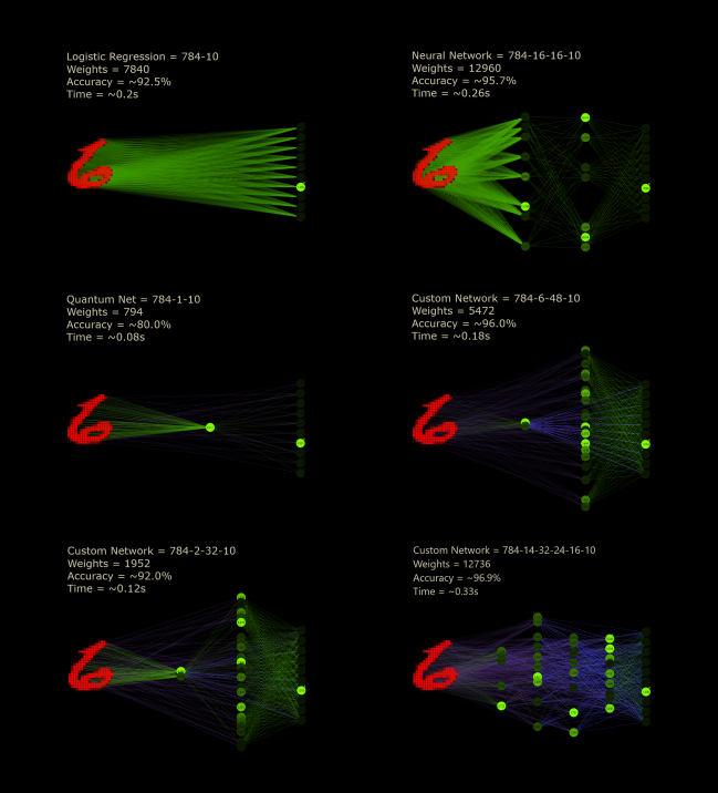
Here are some networks that I trained as best I could. The cc networks were chosen to be below the parameter count of the predecessor networks. Although it's the weakest learner in the round, the quantum net is an exciting design and is different from all other neural networks not only because it's smaller and faster. Incredibly, it uses more neurons than weights. The quantum leap wasn't important because it was supposed to be a big step, but because it refers to the smallest amount of something that you can have.
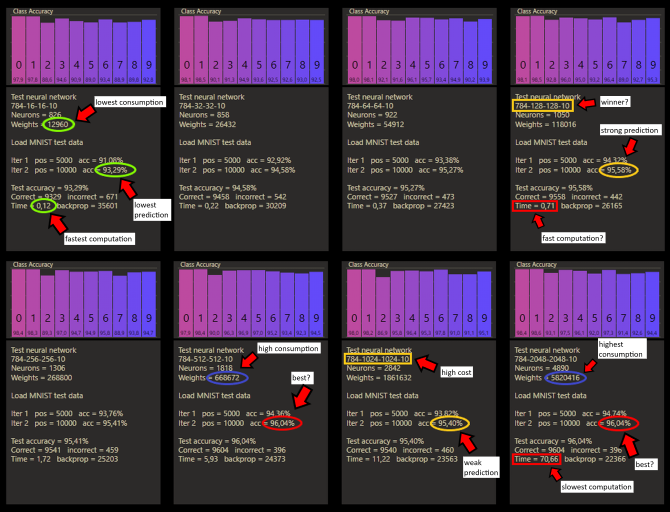
A neural network will always be more efficient than a custom network of the same size. The custom positions are not expensive, but they count. The networks trained above are ordinary neural networks. On the question of efficiency, we could just choose the fastest and smallest network, as above in green. But then the prediction suffers, and that's why we do this. The largest network has the highest prediction, but would consume an incredible amount of memory and computing power by calculating almost 6 million weights.
These results were taken with a better computer, so the times are much faster and larger networks can be tried, but it doesn't seem to be the best decision to just build larger networks for better predictions. First of all, computation time is crucial to develop good systems. Each test more also holds the potential to get closer to higher predictions in my experience. It makes more sense to see which setting has the most potential. Custom connect is very adaptable and efficient exactly in this discipline. My hope is not to build bigger with cc, we should just learn to build right.
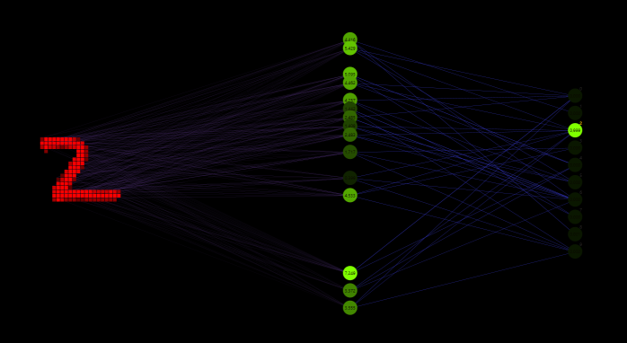
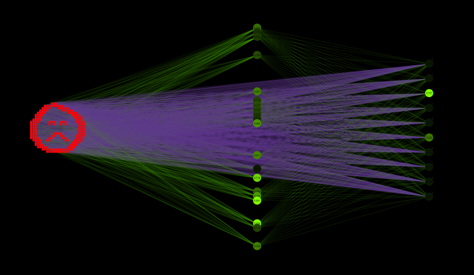
All networks before were still neural networks or mixed networks. But now the green connections are completely gone. The way input neurons connect to hidden neurons or hidden neurons connect to output is again random. These new connections were active before, but now they are 100% active. This 784-5-32-3-10 new net has a jump of 2 and a mix of 100%. The number of neurons on hidden layer 1 determines the density with which the neurons on hidden layer 2 are connected. However, the result is rather just an emulation of this new type of network.
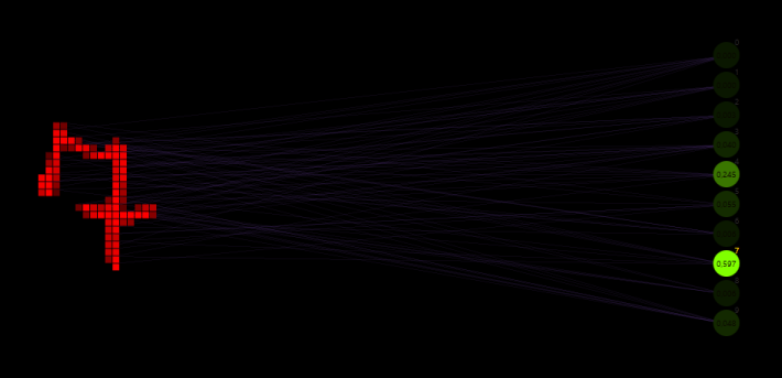
Custom regression could be the right name for this idea, but more importantly, it helps us to make this turn in our heads. Logistic regression with 10 * 784 = 7840 weights distributed over 10 classes with a fully connected pattern would be the smallest linear network. But custom regression shows that we can build 10 times smaller. An image of 784 pixels represented as neurons connected to only one weight each can be sparsely distributed to 10 output neurons and it works pretty well to make predictions. Just a 784-1-10 network with mix = 1 and jump = 2. Remarkable!
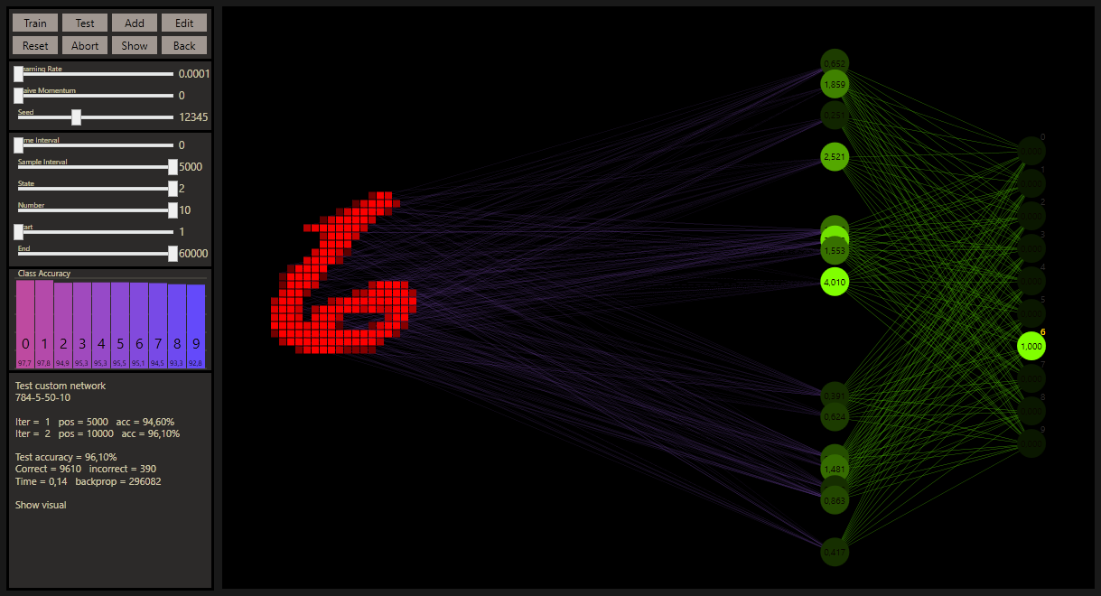
As it turned out, the last layer should be fully connected, otherwise the prediction suffers. The biggest difference to fully connected networks is the much lower density of connections to the hidden neurons in that case. The input neurons connect randomly with input * h1 = 784 * 5 distributed to 50 h2 neurons with a mix of 100% and jump of 2, so that all input to h1 weights are used on h2. However, the fact that the implementation was not actually made for this type of network becomes problematic with more neurons. The connections of h1 * h2 = 5 * 50 = 250 are offline, they are not used effectively. Nevertheless, they occupy memory and are also calculated. The coming considerations will have to take this into account to get a clearer picture about the emulated network.
Unlike previous networks, this type of network requires much higher learning rates to perform well. Learning rates chosen too low lead to even worse predictions than a DNN could do. Adjusted learning rates could help to improve connections of this type. Anyway, for me is this type of network the coolest discovery and therefore the network I will compare against the DNN. The three most important properties in a neural network are prediction accuracy, computation time and memory usage. The accuracy in the test was measured after the networks were fully trained.
| New net | Old net | |
|---|---|---|
| Size | 784-5-50-10 | 784-16-16-10 |
| Accuracy | 96.10% | 95.90% |
| Time | 0.14s | 0.23s |
| Weights | 4670 | 12960 |
It is amazing that an emulation of this network is superior to the old network in every way. The performance is very close to a DNN on a computer twice as fast.
Real memory usage
I will simplify the following calculation to the critical part of memory usage to the weight and its delta array, both have the same length.
In that case the DNN would need at least (weights + deltas) * length = 2 * 12960 = 25920 parameter for a trainable network.
The custom networks need additionally the custom position array with the same length. This yields in (weights + deltas + (custom positions)) * length = 3 * 4670 = 14010 in usage. Further more, better implementations would cut out offline computations by weights - (offline computation) = 4670 - 250 = 4420 and reduce the datatype from int to short for the custom positions array. This would lead to a reduction to (weights + deltas + ((short)custom positions)) * length = 2.5 * 4420 = 11050 in usage.
With a simple click on a neuron, it's possible to customize custom networks even more precisely with a pruned or grown neuron. In technical terms, this is also referred to as structured pruning, or structured growing. When a custom perceptron is pruned that is connected to other neurons, these connections are reset to DNN connections. However, if you have a trained network, as shown in the animation, the connections are preserved, so pruned nodes do not affect the activation levels of the other neurons. At the end of the animation you can see this very nicely, it's also a very good indicator that the algorithm seems to be working correctly so far. Grown nodes are active with a very high probability. The weights can be reinitialized with a reset.
Very nice is that custom connect uses the same optimal way to sort the networks as gg. It may sound a bit crazy, but in principle you could unite all the network structures you have known so far, or whatever else you have in mind. Incredibly complicated algorithm stuff!

One of the ideas was to create really deep neural networks with cc. But what is deep? A neural network with 2 hidden layer is considered to be a deep neural network. It's possible to add more hidden layers, and maybe a 3 layer network could perform better than a 2 layer network, but it could be also possible that a 1 hidden layer neural network outperform the deeper versions. A prediction is hard to make, but for neural networks is that the range I would search on. The hope in the ML community is that with more depth we can generate more intelligent systems. With goodgame, networks with 20 layers could be trained, with good but below average results. That was the limit so far.
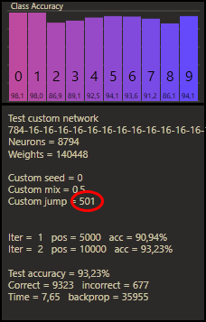
Custom Connect was able to take this idea to a whole new level. The animation above shows a network with 16 hidden neurons on each of the 16 hidden layers. To visually describe the trained ultra-deep net in the figure, we would need 500 hidden layers with 16 neurons. My theory after all the impressions is that with enough hidden neurons we can achieve any depth we want with cc under the technical conditions.
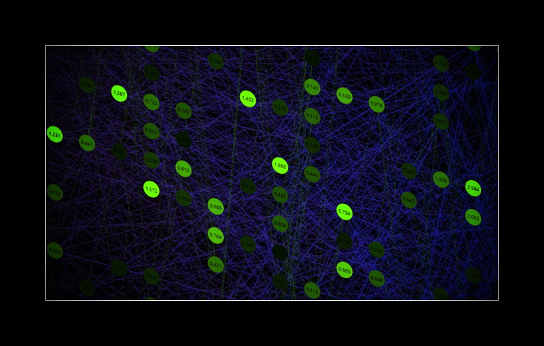
The activation level reveals the secret behind custom connect, which simply goes back to the differential equations, or what is widely known as stochastic gradient descent (SGD). Remember, to change one weight, the entire network must be changed. The weights form a strong team during training. They all start as babies and with the expectation that 50% of the neurons will be activated and 50% will be inactive. The learning rate and the training form these weights in terms of their needs.
The activation levels generated by cc are more balanced than those of a DNN. This is because cc connections bring the connectivity frequency closer to the outputs and increase the density. This then leads to many patterns being detected very early, even directly on connections from the first input to the last output.
The custom connections are the shortcuts to increase learning, connectivity and complexity based on a sparse but well initialized DNN structure, depending on the mix used for cc. Sounds kind of complicated, right? No, it's coming.
The normal way for a DNN would look like this:

First, each input neuron in green is multiplied by its weight in green and added up to the dot product, then the activation function is executed. When the whole layer of perceptrons is processed, the process for the next layer is done in the same way.
With the construction plan of a custom perceptron would a custom network look like this:

The process is basically the same as for the DNN. If the connection is custom, the input times its weight in blue is added as the net input. If the connection is from the DNN, the input times its weight is added to the dot product. Then the net input is added to the dot product and that neuron is activated. Net input and dot product are actually the same thing, but I distinguish here between net input for custom connections and dot product for DNN connections. Both together result in the connected connections to this neuron.
In pseudo-code:
create neural network and feed data

for each layer {
   for each hidden or output neuron {
      for each weight {
         if special weight
            net[customPosition[uniqueKey]] += neuron[inputNeuron] * weight[uniqueKey]; // cc
         else
            dot += neuron[inputNeuron] * weight[uniqueKey]; // dnn
      } // end weight
      dot += net[this]; net[this] = 0;
      neuron[this] = (lastOutputlayer or dot > 0) ? dot : 0;
   } // end neuron
} // end layer
However, the custom connect algorithm is more of a prototype and would be modified at least a bit for upcoming versions.
A backpropagation for the DNN would look like this:

The algorithm starts on the right side and passes each output neuron by taking the difference of target - prediction = error, which is what the partial gradient in red represents. The hidden neurons accumulate from all gradients of the last layer on the right times their weights in green. After the layer is processed, the gradient times the connected input neuron in green on the left gives the delta value in gold to optimize the corresponding weight.
The even more harder step is to understand how custom connect goes back:

Again, the algorithm works in principle the same way as for the DNN, as the last fully connected layer shows. The trick is then to use the delta value loop to accumulate the cc partial gradients in the lower red by calculating the gradient on the right side times the associated cc weight in blue. Once the calculation of the DNN for that neuron is complete, the gradient of the DNN is added to the gradient of the cc until the layer is processed.
After that, the layer for the delta values is calculated by either the already described process for the DNN connection in gold, or for a cc connection in orange. For this, the input neuron in green on the left side is multiplied by the gradient in red on the right side, to which the cc connection points.
In pseudo-code:
for each layer backwards {
   for each output or hidden neuron { // gradients
      if outputLayer
         partialGradient = target == prediction ? 1 - neuron[this] : -neuron[this];
      else {
         for each weight if not special // dnn
            partialGradient += weight[uniqueKey] * gradient[right];
         if not input layer
            for each weight if special // cc
               gradient[left] += weight[uniqueKey] * gradient[customPosition[uniqueKey]];
      }
      gradient[this] += partialGradient;
   } // end neuron
   for each output or hidden neuron { // deltas
      for each weight
         if special // cc
            delta[uniqueKey] += neuron[left] * gradient[customPosition[uniqueKey]];
         else // dnn
            delta[uniqueKey] += neuron[left] * gradient[right];
    } // end neuron
} // end layer
The input gradients are not calculated in this implementation, but they would be needed for a convolutional network in front of custom connect.
This implementation is the resulting compromise of the given requirements. Which leads to the picture you now have in your head. But the picture would look different if, for example, comparability to the old networks had not been one of the requirements. So we have to deal with some of the problems that the compromise brings.
Let me explain, Custom Regression is a good example of where we can run into a trap. The hidden1 neurons represent the connection density. The lowest density is 1, a density of 10 would be the same as logistic regression. You could also use a density of 100, but then you get real problems. There is a strange curve where density improves the prediction for a linear model. But a density above (input * output) seems rather destructive.
A good test to see how much this effect can threaten quality would be the cc network from the Custom Paradox example. If we build this network 10 times larger from 784-16-10 to 784-160-10, the linear density would use 50% of (784 * 160) weights. This would result in poor predictions where a DNN 784-160-10 would significantly outperform the cc accident with the same size.
Another related problem you may have seen is connection conflicts. The cc connections are thrown randomly at neurons and do not take into account whether a connection is already occupied. Other problems, such as the need for higher learning rates on special connections like new net, require even more specialized adaptations. And many challenges are still waiting to be addressed.
It may seem a little intimidating because custom networks look crazy more complex. But maybe you'll get over the initial shock and take a look behind the scenes with me. Actually, there are only three building blocks to understand. A perceptron is a unit of a neural network, at the beginning there is the first perceptron, and at the end there is the last perceptron that the algorithm goes through. Then visualizing and touching the network is another key to see what is going on. With this article, I very much hope to have achieved the goal of making custom networks easy to understand.
All it needs:
perceptron concept +
goodgame +
this
The implementation is based on simplicity and has to do with less rather than more hyperparameters. But of course, there are a lot of details and subtopics that have not been mentioned yet. And many things, like how the console or the network visualization works in detail, are not described. The code can be a guide. But the project consists of several hundred smaller and bigger of these ideas. And to understand all ideas is a huge challenge. Completely without outside help projects like this are often not possible. The visualization is a good example, I had help, but not the kind you would expect. My first visualization attempts were based on this tutorial. The last figure may give you an idea how a neural network can be visualized on it. And many other implementations I had to approximate piece by piece. In an abstract way, the help I used was manageable but necessary.
What I needed:
James D. McCaffrey,
Jörn Loviscach,
MetaQuotes,
StackOverflow,
Youtube
My Equipment:
Visual Studio 2019 Community,
ScreenToGif,
Greenshot,
JPG-Illuminator
Machine learning has been shaped by a wide variety of influences. Data science, statistics, physics and many more. These influences also produced different terms, such as dot product and net input, where weighted sum 1 and weighted sum 2 could also be used. This makes it difficult, especially for beginners, to find their way in this world. The influence for this project comes from e-sports. We are also struggling with terminology, because when a team is thrown together, each player must understand where the called position is, so that the perception of the other team players can be used to advantage. This is what makes good teams.
A major minute of:
e-sports
play hard go pro is the main term to describe what e-sports stands for. That would be my advice if you are willing to take the challenge and learn custom connect. Because my intention was, that even kids can understand that. So no limiting beliefs just because it hurts a little. Max Planck is one of my heroes, you may think of him as you continue your work. About 100 years ago, the biggest misbelief in our world was that energy flows like a river. Under pain, as he said, he had to realize that our world works in portions. Perhaps that is the best advice, to learn cc by portioning it. So far no one can really say how we humans learn. Interesting approaches are the spiral approach and the hermeneutic circle. To close this circle, there is still a piece missing here, play hard after install.
Oh yeah, no bias
There is a bias technique that occurs when the learning process improves by simply suspending updates for too large delta steps until that connection calms down, or not. This biases the node and improves the generalization. This can affect only a single weight, or even all weights. My experiments have confirmed me in dropping the traditional idea of bias for goodgame. This will make the DNN even easier to understand and faster to calculate.
Theoretically, a missing bias can produce worse predictions. In regression problems where a single numerical value must be predicted, this can also be practically problematic. However, in a classification problem such as the prediction of 10 classes of the MNIST dataset a bias seems to be negligible.
- Run Visual Studio 2019 Community
- Download file with MNIST and extract
- Copy the folder with all subdirectories to your c-drive
- Follow the animation (create WPF App, delete stuff, activate Release mode, create cc class, copy code, start cc)
Alternatively, the paths can be changed via code, but the method described is preferred to ensure backward compatibility with gg.
When I was a complete noob in machine learning, someone talked about the idea that the best neural network would simply connect every neuron to every other neuron. The problem is that this isn't possible because even small networks would require an incredible number of connections. So the idea of a compromise was very promising. Maybe that was the reason that inspired me to develop this idea.
The biggest challenge was to implement the idea of custom connections and make them comparable, which led to Perceptron vs. Custom Perceptron. The idea of the classical perceptron is ingenious, but ignores the fact that neural networks always use hidden neurons. When the idea of the perceptron algorithm was presented in 1958, there were no hidden neurons. Custom perceptrons start exactly there.
One of the biggest disadvantages of neural networks is the large amount of training data required. Sample efficiency describes how fast an algorithm can learn. Normally, neural networks need thousands or more training samples to work well. However, since very small custom networks with only a few hundred training samples can predict well, the statement that neural networks are slow learners does not seem to apply to custom networks.
As always with neural networks, in the end there are more questions than answers. Are custom networks also neural networks? When it comes to using techniques like dropout or batch normalization or optimizers like RMSprop or Adam. Then yes. But if you expect the same results as with a neural network, then no!
It was a very cool experience to see what is already in this basic implementation and how well it works. But now it's hard for me to say anything with absolute certainty after all the testing. Except that there is still a lot of room for improvement.
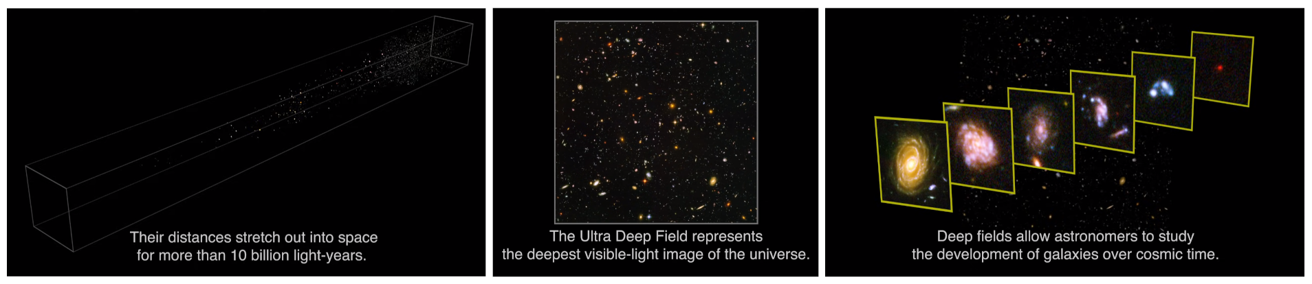
What is deep and how can we measure it? The Doppler effect can be used to determine whether an object is getting closer or moving away. The parallax method allows astronomers to measure the distance of visible objects in space. Hubble's Ultra-Deep Field (HUDF) goes even further. The method used by Hubble is called photometric redshift. But Hubble can't do that alone, so a mix was needed. Center: The once farthest zoom into space. Left: A look back into the past over an incredible span of cosmic time. Right: The growing evolution of galaxies from right to left. Ultra Deep Field: Looking Out into Space, Looking Back into Time.

