- z-Normalization of time series data
- PAA, i.e., Piecewise Aggregate Approximation
- SAX, i.e., Symbolic Aggregate approXimation
- HOT-SAX, an algorithm for the exact time series discord discovery
- VSM, i.e., Vector Space Model
- SAX-VSM, an algorithm for interpretable time series classification (and parameters optimization)
- RePair, an algorithm for grammatical inference
- Rule Density Curve, an efficient grammatical compression (i.e. Kolmogorov Complexity) -based technique for variable length approximate time series anomaly discovery
- RRA (Rare Rule Anomaly), a grammatical compression (i.e. Kolmogorov Complexity) -based algorithm for variable length exact time series anomaly discovery


While RRA was proposed in [8], the code was ported in R to assist for our newer development in SAX parameters optimization: Grammarviz 3.0, please cite it: Senin, P., Lin, J., Wang, X., Oates, T., Gandhi, S., Boedihardjo, A.P., Chen, C., Frankenstein, S., GrammarViz 3.0: Interactive Discovery of Variable-Length Time Series Patterns, ACM Trans. Knowl. Discov. Data, February 2018. [Click here for Citation BibTeX]
In order to process sets of timeseries with uneven length, pad shorter with NA within the input data frame (list). Window-based SAX discretization procedure (sliding window left to right) will detect NA within right side of sliding window and abandon any further processing for the current time series continuing to the next.
[1] Dina Goldin and Paris Kanellakis, On similarity queries for time-series data: Constraint specification and implementation, In Principles and Practice of Constraint Programming – CP ’95, pages 137–153. (1995)
[2] Keogh, E., Chakrabarti, K., Pazzani, M., & Mehrotra, S., Dimensionality reduction for fast similarity search in large time series databases, Knowledge and information Systems, 3(3), 263-286. (2001)
[3] Lonardi, S., Lin, J., Keogh, E., & Patel, P., Finding motifs in time series, In Proc. of the 2nd Workshop on Temporal Data Mining (pp. 53-68). (2002)
[4] Salton, G., Wong, A., Yang., C., A vector space model for automatic indexing, Commun. ACM 18, 11, 613–620, 1975.
[5] Senin Pavel and Malinchik Sergey, SAX-VSM: Interpretable Time Series Classification Using SAX and Vector Space Model., Data Mining (ICDM), 2013 IEEE 13th International Conference on, pp.1175,1180, 7-10 Dec. 2013.
[6] Keogh, E., Lin, J., Fu, A., HOT SAX: Efficiently finding the most unusual time series subsequence, In Proc. ICDM (2005)
[7] N.J. Larsson and A. Moffat. Offline dictionary-based compression., In Data Compression Conference, 1999.
[8] Pavel Senin, Jessica Lin , Xing Wang, Tim Oates, Sunil Gandhi, Arnold P. Boedihardjo, Crystal Chen, Susan Frankenstein, Time series anomaly discovery with grammar-based compression., In Proc. of The International Conference on Extending Database Technology, EDBT 15.
install.packages("devtools")
library(devtools)
install_github('jMotif/jmotif-R')
to start using the library, simply load it into R environment:
library(jmotif)
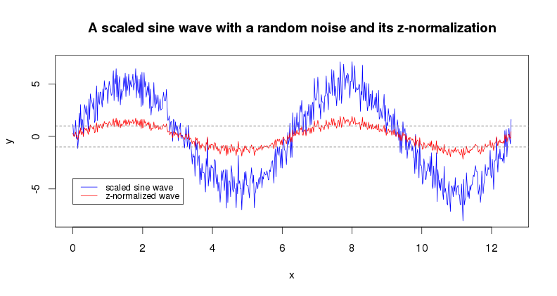
z-normalization (znorm(ts, threshold)) is a common to the field of time series patterns mining preprocessing step proposed by Goldin & Kannellakis which helps downstream analyses to focus on the time series structural features.
x = seq(0, pi*4, 0.02)
y = sin(x) * 5 + rnorm(length(x))

plot(x, y, type="l", col="blue", main="A scaled sine wave with a random noise and its z-normalization")

lines(x, znorm(y, 0.01), type="l", col="red")
abline(h=c(1,-1), lty=2, col="gray50")
legend(0, -4, c("scaled sine wave","z-normalized wave"), lty=c(1,1), lwd=c(1,1),
                                                                col=c("blue","red"), cex=0.8)
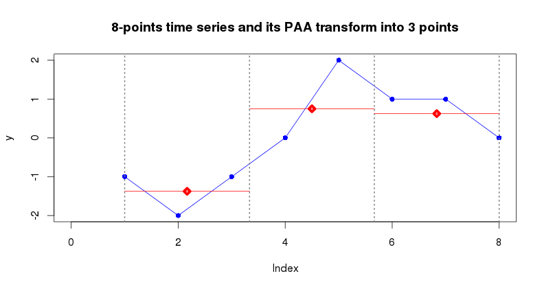
PAA (paa(ts, paa_num)) is designed to reduce the input time series dimensionality by splitting it into equally-sized segments (PAA size) and averaging values of points within each segment. Typically, PAA is applied to z-Normalized time series. In the following example the time series of dimensionality 8 points is reduced to 3 points.
y = c(-1, -2, -1, 0, 2, 1, 1, 0)
plot(y, type="l", col="blue", main="8-points time series and it PAA transform into 3 points")

points(y, pch=16, lwd=5, col="blue")

abline(v=c(1,1+7/3,1+7/3*2,8), lty=3, lwd=2, col="gray50")

y_paa3 = paa(y, 3)

segments(1,y_paa3[1],1+7/3,y_paa3[1],lwd=1,col="red")
points(x=1+7/3/2,y=y_paa3[1],col="red",pch=23,lwd=5)

segments(1+7/3,y_paa3[2],1+7/3*2,y_paa3[2],lwd=1,col="red")
points(x=1+7/3+7/3/2,y=y_paa3[2],col="red",pch=23,lwd=5)

segments(1+7/3*2,y_paa3[3],8,y_paa3[3],lwd=1,col="red")
points(x=1+7/3*2+7/3/2,y=y_paa3[3],col="red",pch=23,lwd=5)
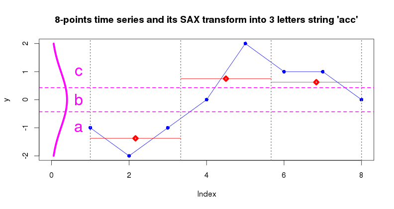
SAX transform (series_to_string(ts, alphabet_size)) is a discretization algorithm which transforms a sequence of rational values (time series points) into a sequence of discrete values - symbols taken from a finite alphabet. This procedure enables the application of numerous algorithms for discrete data analysis to continuous time series data.
Typically, SAX applied to time series of reduced with PAA dimensionality, which effectively yields a low-dimensional, discrete representation of the input time series which preserves (to some extent) its structural characteristics. By employing this representation it is possible to design efficient algorithms for common time series pattern mining tasks as one can rely on the indexing of data in symbolic space. Note, that before processing with PAA and SAX, time series are z-Normalized.
The figure below illustrates the PAA+SAX procedure: 8 points time series is converted into 3-points PAA representation at the first step, PAA values are converted into letters by using 3 letters alphabet at the second step.
y <- seq(-2,2, length=100)
x <- dnorm(y, mean=0, sd=1)
lines(x,y, type="l", lwd=5, col="magenta")
abline(h = alphabet_to_cuts(3)[2:3], lty=2, lwd=2, col="magenta")
text(0.7,-1,"a",cex=2,col="magenta")
text(0.7, 0,"b",cex=2,col="magenta")
text(0.7, 1,"c",cex=2,col="magenta")

> series_to_string(y_paa3, 3)
[1] "acc"

> series_to_chars(y_paa3, 3)
[1] "a" "c" "c"
Another common way to use SAX is to apply the procedure to sliding window-extracted subseries (sax_via_window(ts, win_size, paa_size, alp_size, nr_strategy, n_threshold)). This technique is used in SAX-VSM, where it enables the conversion of a time series into the word bags. Note, the use of a numerosity reduction strategy.
I use the one of standard UCR time series datasets to illustrate the implemented approach. The Cylinder-Bell-Funnel dataset (Saito, N: Local feature extraction and its application using a library of bases. PhD thesis, Yale University (1994)) consists of three time series classes. The dataset is embedded into the jmotif library:
# load Cylinder-Bell-Funnel data
data("CBF")
where it is wrapped into a list of four elements: train and test sets and their labels:
> str(CBF)
List of 4
$ labels_train: num [1:30] 1 1 1 3 2 2 1 3 2 1 ...
$ data_train  : num [1:30, 1:128] -0.464 -0.897 -0.465 -0.187 -1.136 ...
$ labels_test : num [1:900] 2 2 1 2 2 3 1 3 2 3 ...
$ data_test   : num [1:900, 1:128] -1.517 -0.703 -1.412 -0.955 -1.449 ...
At the first step, each class of the training data needs to be transformed into a bag of words using the manyseries_to_wordbag function, which z-normalizes each of time series and converts it into a set of words which added to the resulting bag:
# set the discretization parameters
#
w <- 60 # the sliding window size
p <- 6  # the PAA size
a <- 6  # the SAX alphabet size

# convert the train classes to wordbags (the dataset has three labels: 1, 2, 3)
#
cylinder <- manyseries_to_wordbag(CBF[["data_train"]][CBF[["labels_train"]] == 1,], w, p, a, "exact", 0.01)
bell <- manyseries_to_wordbag(CBF[["data_train"]][CBF[["labels_train"]] == 2,], w, p, a, "exact", 0.01)
funnel <- manyseries_to_wordbag(CBF[["data_train"]][CBF[["labels_train"]] == 3,], w, p, a, "exact", 0.01)
each of these bags is a two-columns data frame:
> head(cylinder)
   words counts
1 aabeee      2
2 aabeef      1
3 aaceee      7
4 aacfee      1
5 aadeee      7
6 aaedde      1
TF*IDF weights are computed at the second step with bags_to_tfidf function which accepts a single argument -- a list of named (by class label) word bags:
# compute tf*idf weights for three bags
#
tfidf = bags_to_tfidf( list("cylinder" = cylinder, "bell" = bell, "funnel" = funnel) )
this yields a data frame of four variables: the words which are "important" in TF*IDF terms (i.e. not presented at least in one of the bags) and their class-corresponding weights:
> tail(tfidf)
     words  cylinder     bell funnel
640 ffcbbb 0.6525709 0.445449 0.0000
641 ffdbab 0.0000000 0.000000 0.7615
642 ffdbbb 1.7681483 0.000000 0.0000
643 ffdcaa 0.0000000 0.000000 0.7615
644 ffdcba 0.0000000 0.000000 0.7615
645 ffebbb 1.5230000 0.000000 0.0000
which makes it easy to find which exact pattern contributes the most to the class:
> library(dplyr)
> head(arrange(tfidf, desc(cylinder)))
   words cylinder bell funnel
1 aaeeee 2.413898    0      0
2 aaceee 2.284500    0      0
3 aadeee 2.284500    0      0

> head(arrange(tfidf, desc(funnel)))
   words cylinder bell   funnel
1 fedcba        0    0 2.975097
2 fedbba        0    0 2.284500
3 adfecb        0    0 1.968449
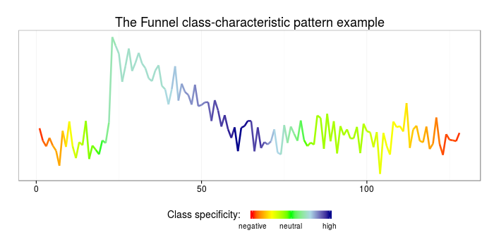
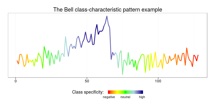
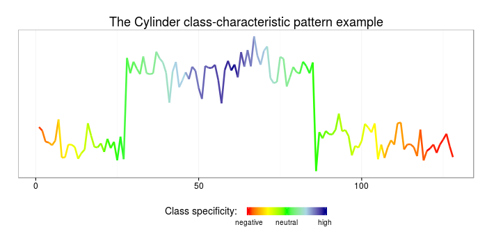
and to visualize those on data:
# make up a sample time-series
#
sample = (CBF[["data_train"]][CBF[["labels_train"]] == 3,])[1,]
sample_bag = sax_via_window(sample, w, p, a, "exact", 0.01)
df = data.frame(index = as.numeric(names(sample_bag)), words = unlist(sample_bag))

# weight the found patterns
#
weighted_patterns = merge(df, tfidf)
specificity = rep(0, length(sample))
for(i in 1:length(weighted_patterns$words)){
  pattern = weighted_patterns[i,]
  for(j in 1:w){
    specificity[pattern$index+j] = specificity[pattern$index+j] +
                                        pattern$funnel - pattern$bell - pattern$cylinder
  }
}

# plot the weighted patterns
#
library(ggplot2)
library(scales)
ggplot(data=data.frame(x=c(1:length(sample)), y=sample, col=rescale(specificity)),
 aes(x=x,y=y,color=col)) + geom_line(size=1.2) + theme_bw() +
 ggtitle("The funnel class-characteristic pattern example") +
 scale_colour_gradientn(name = "Class specificity:  ",limits=c(0,1),
    colours=c("red","yellow","green","lightblue","darkblue"),
    breaks=c(0,0.5,1),labels=c("negative","neutral","high"),
    guide = guide_colorbar(title.theme=element_text(size=14, angle=0),title.vjust=1,
    barheight=0.6, barwidth=6, label.theme=element_text(size=10, angle=0))) +
 theme(legend.position="bottom",plot.title=element_text(size=18),
    axis.title.x=element_blank(), axis.title.y=element_blank(),
    axis.text.x=element_text(size=12),axis.text.y=element_blank(),
    panel.grid.major.y = element_blank(), panel.grid.minor.y = element_blank(),
    axis.ticks.y = element_blank())
Using the weighted patterns obtained at the previous step and the cosine similarity measure it is also easy to classify unlabeled data using the cosine_sim function which accepts a list of two elements: the bag-of-words representation of the input time series (constructed with series_to_wordbag function) and the TF*IDF weights table obtained at the previous step:
# classify the test data
#
labels_predicted = rep(-1, length(CBF[["labels_test"]]))
labels_test = CBF[["labels_test"]]
data_test = CBF[["data_test"]]
for (i in c(1:length(data_test[,1]))) {
    series = data_test[i,]
    bag = series_to_wordbag(series, w, p, a, "exact", 0.01)
    cosines = cosine_sim(list("bag"=bag, "tfidf" = tfidf))
    labels_predicted[i] = which(cosines$cosines == max(cosines$cosines))
}

# compute the classification error
#
error = length(which((labels_test != labels_predicted))) / length(labels_test)
error

# findout which time series were misclassified
#
which((labels_test != labels_predicted))
Here I shall show how the classification task discretization parameters optimization can be done with third-party libraries, specifically nloptr which implements DIRECT and cvTools which facilitates CV process. But not forget the magic of plyr!!! So here is the code:
library(plyr)
library(cvTools)
library(nloptr)

# the cross-validation error function
# uses the following global variables
#   1) nfolds -- specifies folds for the cross-validation
#                if equal to the number of instances, then it is
#                LOOCV
#
cverror <- function(x) {

  # the vector x suppos to contain reational values for the
  # discretization parameters
  #
  w = round(x[1], digits = 0)
  p = round(x[2], digits = 0)
  a = round(x[3], digits = 0)

  # few local vars to simplify the process
  m <- length(train_labels)
  c <- length(unique(train_labels))
  folds <- cvFolds(m, K = nfolds, type = "random")

  # saving the error for each folds in this array
  errors <- list()

  # cross-valiadtion business
  for (i in c(1:nfolds)) {

    # define data sets
    set_test <- which(folds$which == i)
    set_train <- setdiff(1:m, set_test)

    # compute the TF-IDF vectors
    bags <- alply(unique(train_labels),1,function(x){x})
    for (j in 1:c) {
      ll <- which(train_labels[set_train] == unique(train_labels)[j])
      bags[[unique(train_labels)[j]]] <-
        manyseries_to_wordbag( (train_data[set_train, ])[ll,], w, p, a, "exact", 0.01)
    }
    tfidf = bags_to_tfidf(bags)

    # compute the eror
    labels_predicted <- rep(-1, length(set_test))
    labels_test <- train_labels[set_test]
    data_test <- train_data[set_test,]

    for (j in c(1:length(labels_predicted))) {
      bag=NA
      if (length(labels_predicted)>1) {
        bag = series_to_wordbag(data_test[j,], w, p, a, "exact", 0.01)
      } else {
        bag = series_to_wordbag(data_test, w, p, a, "exact", 0.01)
      }
      cosines = cosine_sim(list("bag" = bag, "tfidf" = tfidf))
      if (!any(is.na(cosines$cosines))) {
        labels_predicted[j] = which(cosines$cosines == max(cosines$cosines))
      }
    }

    # the actual error value
    error = length(which((labels_test != labels_predicted))) / length(labels_test)
    errors[i] <- error
  }

  # output the mean cross-validation error as the result
  err = mean(laply(errors,function(x){x}))
  print(paste(w,p,a, " -> ", err))
  err
}

# define the data for CV
train_data <- CBF[["data_train"]]
train_labels <- CBF[["labels_train"]]
nfolds = 15

# perform the parameters optimization
S <- directL(cverror, c(10,2,2), c(120,60,12),
             nl.info = TRUE, control = list(xtol_rel = 1e-8, maxeval = 10))
The optimization process goes as follows:
[1] "65 31 7  ->  1"
[1] "65 31 7  ->  1"
[1] "65 31 7  ->  1"
[1] "28 31 7  ->  1"
[1] "102 31 7  ->  1"
[1] "65 12 7  ->  0.366666666666667"
[1] "65 50 7  ->  1"
[1] "65 31 4  ->  1"
[1] "65 31 10  ->  1"
[1] "28 12 7  ->  0.833333333333333"
[1] "102 12 7  ->  0.666666666666667"
[1] "65 12 4  ->  0"

Call:
nloptr(x0 = x0, eval_f = fn, lb = lower, ub = upper, opts = opts)
Minimization using NLopt version 2.4.2

NLopt solver status: 5 ( NLOPT_MAXEVAL_REACHED: Optimization stopped because maxeval (above) was
reached. )

Number of Iterations....: 10
Termination conditions:  stopval: -Inf xtol_rel: 1e-08 maxeval: 10 ftol_rel: 0 ftol_abs: 0
Number of inequality constraints:  0
Number of equality constraints:    0
Current value of objective function:  0
Current value of controls: 65 11.66667 3.666667
At this point S contains the best SAX parameters which were found using 10 DIRECT iterations, which we can use for the classification of the test data:
w = round(S$par[1], digits = 0)
p = round(S$par[2], digits = 0)
a = round(S$par[3], digits = 0)

# compute the TF-IDF vectors
#
bags <- alply(unique(train_labels),1,function(x){x})
for (j in 1:length(unique(train_labels))) {
  ll <- which(train_labels == unique(train_labels)[j])
  bags[[unique(train_labels)[j]]] <-
    manyseries_to_wordbag( train_data[ll,], w, p, a, "exact", 0.01)
}
tfidf = bags_to_tfidf(bags)

# classify the test data
#
labels_predicted = rep(-1, length(CBF[["labels_test"]]))
labels_test = CBF[["labels_test"]]
data_test = CBF[["data_test"]]
for (i in c(1:length(data_test[,1]))) {
  print(paste(i))
  series = data_test[i,]
  bag = series_to_wordbag(series, w, p, a, "exact", 0.01)
  cosines = cosine_sim(list("bag"=bag, "tfidf" = tfidf))
  if (!any(is.na(cosines$cosines))) {
    labels_predicted[i] = which(cosines$cosines == max(cosines$cosines))
  }
}

# compute the classification error
#
error = length(which((labels_test != labels_predicted))) / length(labels_test)
error

# findout which time series were misclassified
#
which((labels_test != labels_predicted))
par(mfrow=c(3,1))
plot(data_test[316,], type="l")
plot(data_test[589,], type="l")
plot(data_test[860,], type="l")
which shows us that one instance of each of the classes was misclassified....
Given a time series T, its subsequence C is called discord if it has the largest Euclidean distance to its nearest non-self match. Thus, time series discord is a subsequence within a time series that is maximally different to all the rest of subsequences in the time series, and therefore naturally captures the most unusual subsequence within the time series.
The library embeds the ECG0606 dataset taken from PHYSIONET FTP. The raw data was transformed with their rdsamp utility
rdsamp -r sele0606 -f 120.000 -l 60.000 -p -c | sed -n '701,3000p' >0606.csv
and consists of 15 heartbeats:
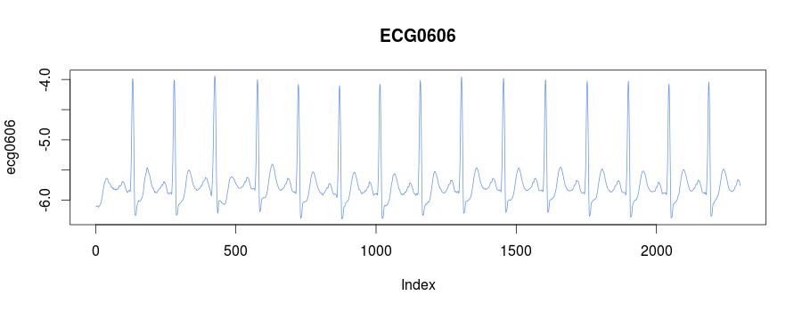
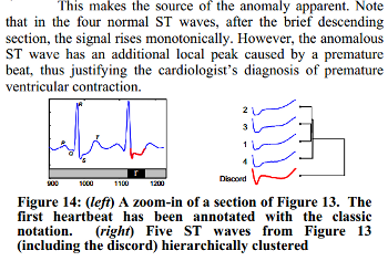
We know, that the third heartbeat of this dataset contains the true anomaly as it was discussed in HOTSAX paper by Eamonn Keogh, Jessica Lin, and Ada Fu. Note, that the authors were specifically interested in finding anomalies which are shorter than a regular heartbeat following a suggestion given by the domain expert: ''We conferred with cardiologist, Dr. Helga Van Herle M.D., who informed us that heart irregularities can sometimes manifest themselves at scales significantly shorter than a single heartbeat.'' Figure 13 of the paper further explains the nature of this true anomaly:
Two implementation of discord discovery provided within the code: the brute-force discord discovery and HOT-SAX.
The brute-force takes 14 seconds to discover 5 discords in the data (with early-abandoning distance):
> lineprof( find_discords_brute_force(ecg0606, 100, 5) )
Reducing depth to 2 (from 18)
    time    alloc  release dups                    ref            src
1 13.951 6211.306 6209.214    2                ".Call" .Call
2  0.001    0.000    0.000   44 c(".Call", "tryCatch") .Call/tryCatch
whereas HOT-SAX finishes in fraction of a second:
> lineprof( find_discords_hotsax(ecg0606, 100, 4, 4, 0.01, 5) )
   time alloc release dups     ref   src
1 0.191 0.245       0   56 ".Call" .Call
The discords returned as a data frame sorted by the position:
> discords = find_discords_hotsax(ecg0606, 100, 4, 4, 0.01, 5)
> discords
  nn_distance position
1   0.4787745       37
2   0.4177020      188
3   1.5045847      411
4   0.4437060      539
5   0.4437060     1566
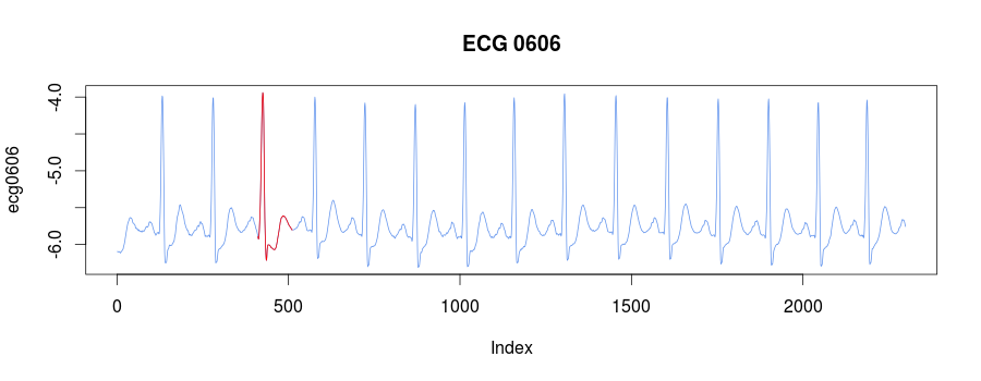
The best discord is the third one at 411:
discords = find_discords_hotsax(ecg0606, 100, 4, 4, 0.01, 5)
plot(ecg0606, type = "l", col = "cornflowerblue", main = "ECG 0606")
lines(x=c(discords[3,2]:(discords[3,2]+100)),
    y=ecg0606[discords[3,2]:(discords[3,2]+100)], col="red")
It is easy to sort discord by the nearest neighbor distance:
> library(dplyr)
> arrange(discords,desc(nn_distance))
  nn_distance position
1   1.5045847      411
2   0.4787745       37
3   0.4437060      539
4   0.4437060     1566
5   0.4177020      188
RePair is a dictionary-based compression method proposed in 1999 by Larsson and Moffat. In contrast with Sequitur, Repair is an off-line algorithm that requires the whole input sequence to be accessible before building a grammar. Similar to Sequitur, RePair also can be utilized as a grammar-based compressor able to discover a compact grammar that generates the text. It is a remarkably simple algorithm which is known for its very fast decompression.
In short, RePair performs a recursive pairing step -- finding the most frequent pair of symbols in the input sequence and replacing it with a new symbol -- until every pair appears only once.
As noted by the authors, when compared with online compression algorithms, the disadvantage of Repair having to store a large message in memory for processing is illusory when compared with storing the growing dictionary of an online compressor, as the incremental dictionary-based algorithms maintain an equally large message in memory as a part of the dictionary.
Here is an example of RePair grammar for the input string containing an anomaly (xxx). Note that none of the grammar rules includes the anomalous terminal symbol.
Grammar rule        Expanded grammar rule                        Occurrence in R0
R0 -> R4 xxx R4     abc abc cba cba bac xxx abc abc cba cba bac
R1 -> abc abc       abc abc                                      2-3, 8-9
R2 -> cba cba       cba cba                                      0-1, 6-7
R3 -> R1 R2         abc abc cba cba                              0-3, 6-9
R4 -> R3 bac        abc abc cba cba bac                          0-4, 6-10
Calling RePair implementation in jmotif-R
grammar <- str_to_repair_grammar("abc abc cba cba bac xxx abc abc cba cba bac")
produces a list of data frames, each of which contains the RePair grammar rule information. For example the first rule of the grammar (second list element):
> str(grammar[[2]])
List of 5
 $ rule_name           : chr "R1"
 $ rule_string         : chr "cba cba"
 $ expanded_rule_string: chr "cba cba"
 $ rule_interval_starts: num [1:2] 2 8
 $ rule_interval_ends  : num [1:2] 3 9
As we have discussed in our work, SAX opens door for many high-level string algorithms application to the problem of patterns mining in time series. Specifically in [8], we have shown useful properties of grammatical compression (i.e., algorithmic complexity) when applied to the problem of recurrent and anomalous pattern discovery.
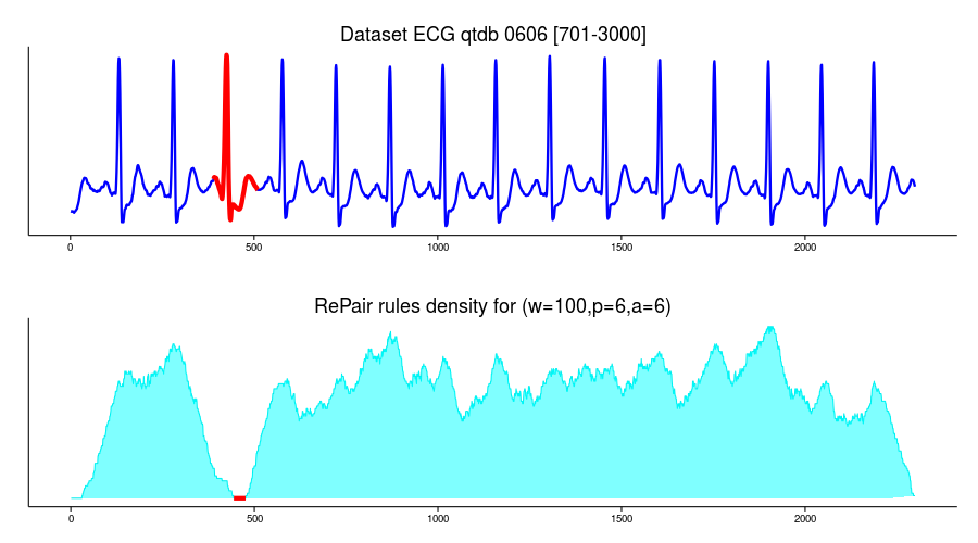
Jmotif-R implements RePair [7] algorithm for grammar induction, which can be used to build the rule density curve enabling highly efficient approximate time series anomaly discovery.
I use the same ECG0606 dataset in this example:
ecg <- ecg0606

require(ggplot2)
df=data.frame(time=c(1:length(ecg)),value=ecg)
p1 <- ggplot(df, aes(time, value)) + geom_line(lwd=1.1,color="blue1") + theme_classic() +
  ggtitle("Dataset ECG qtdb 0606 [701-3000]") +
  theme(plot.title = element_text(size = rel(1.5)),
    axis.title.x = element_blank(),axis.title.y=element_blank(),
    axis.ticks.y=element_blank(),axis.text.y=element_blank())
p1
and use RePair implementation to build the grammar curve:
# discretization parameters
w=100
p=8
a=8

# discretize the data
ecg_sax <- sax_via_window(ecg, w, p, a, "none", 0.01)

# get the string representation of time series
ecg_str <- paste(ecg_sax, collapse=" ")

# infer the grammar
ecg_grammar <- str_to_repair_grammar(ecg_str)

# initialize the density curve
density_curve = rep(0,length(ecg))

# account for all the rule intervals
for(i in 2:length(ecg_grammar)){
    rule = ecg_grammar[[i]]
    for(j in 1:length(rule$rule_interval_starts)){
        xs = rule$rule_interval_starts[j]
        xe = rule$rule_interval_ends[j] + w
        density_curve[xs:xe] <- density_curve[xs:xe] + 1;
    }
}

# see global minimas
which(density_curve==min(density_curve))
# [1]   1   2   3   4   5   6   7   8   9  10  11  12  13  14  15  16  17  18  19  20  21  22  23  24
# [25]  25  26  27  28  29  30 444 445 446 447 448 449 450 451 452 453 454 455 456 457 458 459 460 461
# [49] 462 463 464 465 466 467 468 469 470 471 472 473 474 475 476
min_values = data.frame(x=c(444:476),y=rep(0,(476-443)))

# plot the curve
density_df=data.frame(time=c(1:length(density_curve)),value=density_curve)
shade <- rbind(c(0,0), density_df, c(2229,0))
names(shade)<-c("x","y")
p2 <- ggplot(density_df, aes(x=time,y=value)) +
    geom_line(col="cyan2") + theme_classic() +
    geom_polygon(data = shade, aes(x, y), fill="cyan", alpha=0.5) +
    ggtitle("RePair rules density for (w=100,p=8,a=8)") +
    theme(plot.title = element_text(size = rel(1.5)), axis.title.x = element_blank(),
    axis.title.y=element_blank(), axis.ticks.y=element_blank(),axis.text.y=element_blank())+
    geom_line(data=min_values,aes(x,y),lwd=2,col="red")
p2

grid.arrange(p1, p2, ncol=1)
RRA (i.e., Rare Rule Anomaly) algorithm extends the HOT-SAX algorithm leveraging the grammatical compression properties (i.e. algorithmic, or Kolmogorov complexity properties). In contrast with the original algorithm, whose input is a set of time series subsequences extracted from the input time series via sliding window, RRA operates on the set of time series subsequences which correspond to a grammar' rules. The grammar, whose rules are used in RRA, is built by a grammar inference algorithm run on the set of tokens which are obtained by time series discretization with SAX and a sliding window (i.e. a HOT-SAX input). jmotif-R is using Re-Pair algorithm for grammatical inference.
Since each of the grammar rules consists of terminal and non-terminal tokens, the subsequences corresponding to rules naturally vary in length. Moreover, due to the compression properties of the utilized grammatical inference algorithm, which operates on digrams (i.e. pairs of subsequences extracted via sliding window), the amount of input subsequences for RAA is usually significantly lower than those extracted via sliding window for HOT-SAX, which improves the efficiency of HOT-SAX inner and outer loops by reducing the number of calls to the distance function.
In addition to the above, RRA uses a different heuristics for the ordering in the HOT-SAX outer loop: instead of ordering subsequences by their occurrence frequency, the rule-corresponding subsequences are ordered according to the "rule coverage" values discussed above -- a value which reflects the compressibility of the subsequence. Naturally, we expect that incompressible subsequences correspond to potential anomalies.