GithubHelp home page GithubHelp logo

juliarobotics / kerneldensityestimate.jl Goto Github PK

View Code? Open in Web Editor NEW
23.0 4.0 7.0 655 KB

Kernel Density Estimate with product approximation using multiscale Gibbs sampling

License: GNU Lesser General Public License v2.1

Julia 100.00%
multiscale-gibbs-sampling probabilistic-programming bayesian inference julialang gadfly

kerneldensityestimate.jl's Introduction

KernelDensityEstimate.jl

CI codecov.io

Kernel Density Estimation with product approximation using multiscale Gibbs sampling.

All code is implemented in native Julia, including plotting. The main focus of this module is the ability to take the product between multiple KDEs, and makes this module unique from other KDE implementations. This package also supports n-dimensional KDEs. Please see examples below for details. The implementation is already fairly optimized from a symbolic standpoint and is based on work by:

Sudderth, Erik B.; Ihler, Alexander, et al. "Nonparametric belief propagation." Communications of the ACM 53.10 (2010): 95-103.

Installation

In Julia 1.0 and above:

] add KernelDensityEstimate

Plotting Functions

The plotting functions for this library have been separated into KernelDensityEstimatePlotting.jl. Plotting functionality uses Gadfly. Comments welcome.

Examples

Bring the module into the workspace

using KernelDensityEstimate
# Basic one dimensional examples
# using leave-one-out likelihood cross validation for bandwidth estimation
p100 = kde!([randn(50);10.0.+2*randn(50)])
p2 = kde!([0.0;10.0],[1.0]) # multibandwidth still to be added
p75 = resample(p2,75)

# bring in the plotting functions
using KernelDensityEstimatePlotting
plot([p100;p2;p75],c=["red";"green";"blue"]) # using Gadfly under the hood

alt tag

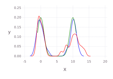
Multidimensional example

pd2 = kde!(randn(3,100));
@time pd2 = kde!(randn(3,100)); # defaults to loocv
pm12 = marginal(pd2,[1;2]);
pm2 = marginal(pm12,[2]);
plot(pm2);

Multiscale Gibbs product approximation example

p = kde!(randn(2,100))
q = kde!(2.0.+randn(2,100))
dummy = kde!(rand(2,100),[1.0]);
mcmciters = 5
pGM, = prodAppxMSGibbsS(dummy, [p;q], nothing, nothing, Niter=mcmciters)
pq = kde!(pGM)
pq1 = marginal(pq,[1])
Pl1 = plot([marginal(p,[1]);marginal(q,[1]);marginal(pq,[1])],c=["red";"green";"black"])

Direct histogram of points from the product

using Gadfly
Pl2 = Gadfly.plot(x=pGM[1,:],y=pGM[2,:],Geom.histogram2d);
draw(PDF("product.pdf",15cm,8cm),hstack(Pl1,Pl2))

alt tag

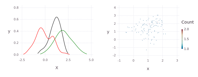
KDE product between non-gaussian distributions

using Distributions
p = kde!(rand(Beta(1.0,0.45),300));
q = kde!(rand(Rayleigh(0.5),100).-0.5);
dummy = kde!(rand(1,100),[1.0]);
pGM, = prodAppxMSGibbsS(dummy, [p;q], nothing, nothing, Niter=5)
pq = kde!(pGM)
plot([p;q;pq],c=["red";"green";"black"])

alt tag

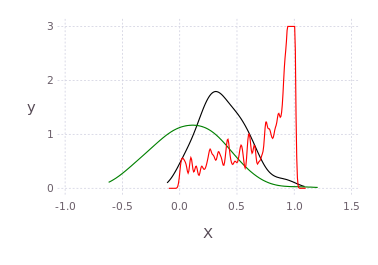
Draw multidimensional distributions as marginalized 2D contour plots

axis=[[-5.0;5]';[-2.0;2.0]';[-10.0;10]';[-5.0;5]']
draw(PDF("test.pdf",30cm,20cm),
 plot( kde!(randn(4,200)) ) )

N=200;
pts = [2*randn(1,N).+3;
 [2*randn(1,round(Int,N/2))'.+3.0;2*randn(1,round(Int,N/2))'.-3.0]';
 2*randn(2,N).+3];
p, q = kde!(randn(4,100)), kde!(pts);
draw(PNG("MultidimPlot.png",15cm,10cm),
 plot( [p*q;p;q],c=["red";"black";"blue"], axis=axis, dims=2:4,dimLbls=["w";"x";"y";"z"], levels=4) )

alt tag

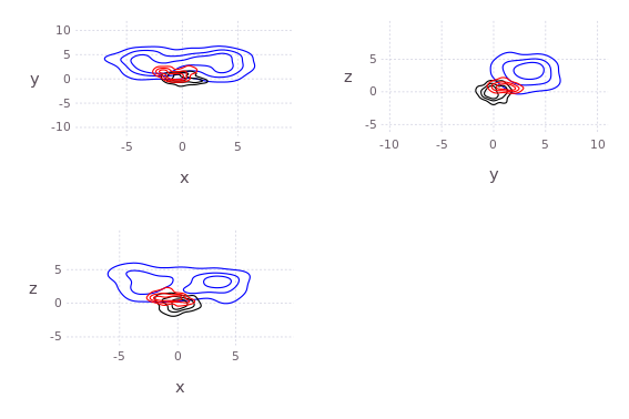
# or draw product natively
draw(PNG("MultidimPlotProd.png",10cm,7cm),
 plot( p*q, axis=axis, dims=[2;4],dimLbls=["w";"x";"y";"z"]) )

alt tag

Contributors

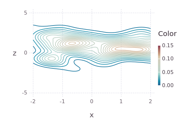
The original C++ kde package was written by Alex Ihler and Mike Mandel in 2003, and has be rewritten in Julia and continuously modified by Dehann Fourie since.

Thank you to contributors and users alike, comments and improvements welcome according to JuliaLang and JuliaRobotics standards.

kerneldensityestimate.jl's People

Contributors

affie avatar andreasnoack avatar dehann avatar github-actions[bot] avatar juliatagbot avatar

Stargazers

 avatar  avatar  avatar  avatar  avatar  avatar  avatar  avatar  avatar  avatar  avatar  avatar  avatar  avatar  avatar  avatar  avatar  avatar  avatar  avatar  avatar  avatar  avatar

Watchers

 avatar  avatar  avatar  avatar

kerneldensityestimate.jl's Issues

Separate plotting

Functionality should continue to work, since plotting requires much more user infrastructure.

Maybe a separate package like:

KernelDensityPlotting.jl

Will be useful for all three the KDE* .jl packages out there. Have 1D, and several 2D for multidimensional, as well as contour density evaluation.

cc @wadehenning (as FYI)

Native Integer Size

Throughout the code integers are represented as Int64.
This causes problems on 32 bit machines for example

    n::Int64
    reshape(M, n, 1)

The 1 is interpreted as a Int32 giving an error of no method found for reshape(::Array, ::Int64, ::Int32)
I would suggest using Int as it represents either Int32 or Int64 depending on native format.
Of course only where Int32 is large enough to represent the number, arrays of length 2e9 might take a bit long to compute on an small processor in any case :-)
I changed it as a test to get KernelDensityEstimates running on a raspberry pi

Function Usage

Hi @dehann.
I am mostly interested in finding the likelihood that a given random variable is a member of a sample (for both scalar valued and multivariate random variables). This seems to be what you are plotting in your examples, but I can't unpack how you arrive at those values. Using the 'calcStatsHandle' perhaps?

I am also interested in your product approximation. How do you interpret this product? It looks like the average of the densities...

Thank You,
Wade

Reuse Bandwidth or Density

Once I estimate a density for a set of training points I would like to be able to store the density and have it available for classification of new test points. My current approach for estimating likelihoods looks something like:

pNormal = kde!(randn(2,10000))
sampleNormal = resample(pNormal, 1000)
likelihoods = evaluateDualTree(pNormal,sampleNormal)

But estimating the density every time I need it is too slow for multiple large data sets in real time. In looking at the BallTreeDensity, it seems that there is no way for me to store the whole density estimate (in a database) for later use. However, I suspect most of the kde! calculation time is spend on the LOOCV bandwidth estimation. Is there a way for me to store the bandwidth and reuse it on subsequent calls to kde!() based on the same training data?

Thanks for any thoughts.

what does the function kde! modify?

By convention in Julia, a function that ends with ! modifies some of its input arguments.

It seems like kde! can be called with only the data for the estimation. Does the function modify the input data? If so, it'd be great to clarify on the usage case and give an option that doesn't modify the input data

Access Sampled Points

In the resample() function, how do you get access to the actual sampled points from the returned BallTreeDensity? In the code below, I need the actual 75 points that were sampled from the density.

p2 = kde!([0.0;10.0],[1.0]) # multibandwidth still to be added
p75 = resample(p2,75)

Thanks in advance!

remove Fontconfig dependency?

I am very interested in trying your KernelDensityEstimate package, but I am having trouble loading Fontconfig on my Windows machine. If I fork this and remove the KDEPlotting01.jl file, will this eliminate the need for the dependencies? Your plots look great and I would like to try them, I am most interested in the numerical results.

Thanks,
Wade

Warning: Error requiring Fontconfig from Compose:

$ julia ./kerneldensity.jl
┌ Warning: Error requiring Fontconfig from Compose:
│ LoadError: UndefVarError: Cairo not defined
│ Stacktrace:
│  [1] top-level scope at /home/lxc/.julia/packages/Compose/Opbga/src/pango.jl:3
│  [2] include(::Module, ::String) at ./Base.jl:377
│  [3] include(::String) at /home/lxc/.julia/packages/Compose/Opbga/src/Compose.jl:1
│  [4] top-level scope at /home/lxc/.julia/packages/Compose/Opbga/src/Compose.jl:176
│  [5] eval at ./boot.jl:331 [inlined]
│  [6] eval at /home/lxc/.julia/packages/Compose/Opbga/src/Compose.jl:1 [inlined]
│  [7] (::Compose.var"#119#125")() at /home/lxc/.julia/packages/Requires/9Jse8/src/require.jl:67
│  [8] err(::Compose.var"#119#125", ::Module, ::String) at /home/lxc/.julia/packages/Requires/9Jse8/src/require.jl:38
│  [9] #118 at /home/lxc/.julia/packages/Requires/9Jse8/src/require.jl:66 [inlined]
│  [10] withpath(::Compose.var"#118#124", ::String) at /home/lxc/.julia/packages/Requires/9Jse8/src/require.jl:28
│  [11] #117 at /home/lxc/.julia/packages/Requires/9Jse8/src/require.jl:65 [inlined]
│  [12] listenpkg(::Compose.var"#117#123", ::Base.PkgId) at /home/lxc/.julia/packages/Requires/9Jse8/src/require.jl:13
│  [13] macro expansion at /home/lxc/.julia/packages/Requires/9Jse8/src/require.jl:64 [inlined]
│  [14] __init__() at /home/lxc/.julia/packages/Compose/Opbga/src/Compose.jl:175
│  [15] _include_from_serialized(::String, ::Array{Any,1}) at ./loading.jl:697
│  [16] _require_search_from_serialized(::Base.PkgId, ::String) at ./loading.jl:781
│  [17] _tryrequire_from_serialized(::Base.PkgId, ::UInt64, ::String) at ./loading.jl:712
│  [18] _require_search_from_serialized(::Base.PkgId, ::String) at ./loading.jl:770
│  [19] _require(::Base.PkgId) at ./loading.jl:1006
│  [20] require(::Base.PkgId) at ./loading.jl:927
│  [21] require(::Module, ::Symbol) at ./loading.jl:922
│  [22] include(::Module, ::String) at ./Base.jl:377
│  [23] exec_options(::Base.JLOptions) at ./client.jl:288
│  [24] _start() at ./client.jl:484
│ in expression starting at /home/lxc/.julia/packages/Compose/Opbga/src/pango.jl:3
└ @ Requires ~/.julia/packages/Requires/9Jse8/src/require.jl:40

My kerneldensity.jl

using JLD2, KernelDensityEstimate, KernelDensityEstimatePlotting
@load "seasontop.jld2" spri_tops
p = kde!(convert(Vector{Float64},spri_tops))
plot(p)

spri_tops is a 1-d Array of Float32, so I convert it to Float64.

option to specify bounds on plotKDE

Hi, I was wondering if the rmin/rmax properties can be reinstated into the plotting options? Or if there's a workaround?
I'm trying to look at a 1D density on [0,1] and no matter what I try, the x-axis defaults to [0,15] (odd enough, considering my data was in [0,1] to begin with), so I cannot actually tell what is going on in my region of interest.

Otherwise, love the plotting functionality.

Get conditional kernel densities

Hello,

This may be more of a discussion topic, but I post it here as perhaps discussions have not been activated yet in this repo, and it could be more appropriate to have this here rather than on the discourse.

I was wondering if there is a method to get a conditional distribution out of a ::BallTreeDensity.

So say for example that I have the following code:

using KernelDensityEstimate, Distributions

# define number of samples
const n_samples = 500

# define two correlated variables
const x = randn(n_samples)
const y = x.^2 .+ rand(Uniform(-0.0005, 0.0005), n_samples) 

# and an uncorrelated one
const z = rand(Gamma(), n_samples);

# fit the kde
kde = kde!(Array((hcat(x,y,z)')))

And I would like to get the distribution of x and y conditioned to, say, z = 10.

How would you do it?

Thank you very much

How to do plotting with 'KernelDensityEstimatePlotting.jl'?

Is it possible to plot without 'KernelDensityEstimatePlotting.jl'?

Could some more examples be presented in the readme? It would be great if some of the examples could present how to derive the values of the density returned from kde! over a range.

change license to MIT (or GPL)?

I was looking for LGPL packages, suspecting that there should not be many since for a Julia package there's no such thing as "linking" making LGPL equivalent to GPL. Since I suspect the intention is not to have a viral license I thought I'd ask about changing the license to MIT, which should be possible since there aren't that many contributors. If the intention is to have a viral license, then you could leave it as-is, but you could also make that more explicit by changing the license to GPL, although that seems unlikely to be worth the effort.

Better dispatch on evaluations

This and all related ::AbstractArray{<:Real}, also towards AD, e.g.

julia> p1(-2:0.1:2)
ERROR: MethodError: no method matching (::BallTreeDensity)(::StepRangeLen{Float64, Base.TwicePrecision{Float64}, Base.TwicePrecision{Float64}})
Closest candidates are:
  (::BallTreeDensity)(::Vector{Float64}) at /home/dehann/.julia/packages/KernelDensityEstimate/Kx5zN/src/DualTree01.jl:438

julia> p3(v')
ERROR: MethodError: no method matching (::BallTreeDensity)(::LinearAlgebra.Adjoint{Float64, Matrix{Float64}})
Closest candidates are:
  (::BallTreeDensity)(::Vector{Float64}) at /home/dehann/.julia/packages/KernelDensityEstimate/Kx5zN/src/DualTree01.jl:438

Stand-alone sampling

What is the recommended method for using the Gibbs sampler to draw samples from a fit density estimate (independent of any plotting, products, etc)? I would assume this functionality exists in somewhere in MSGibbs01.jl, I just haven't been able to isolate it.

Get the bandwidth

Hello,
I like this package so much,but I don't know how can I get the bandwidth calculated by kde! .

TagBot trigger issue

This issue is used to trigger TagBot; feel free to unsubscribe.

If you haven't already, you should update your TagBot.yml to include issue comment triggers.
Please see this post on Discourse for instructions and more details.

If you'd like for me to do this for you, comment TagBot fix on this issue.
I'll open a PR within a few hours, please be patient!

only selecting first element during 1-product?

MWE

pts = randn(5)
p_ = *([kde!(pts);], addEntropy=false)

pts_ = getPoints(p_)
# results in 5 values all equal to pts[1]
@assert pts_[2] != pts[2] "points in product of [p;] should be identical to original points"

Likely something to do with:

glb.particles[dim,j] = mean(glb.trees[j], glb.ind[j], dim)

and used here:

glb.calcmu[j] = glb.particles[dim,j] #[dim+glb.Ndim*(j-1)]

and closest to user:

How to modify the kernel ?

Hi,
I couldn't figure out how to modify the kernel. In particular, I would like to be able to compute gradients of the density.
Thank you,

Nadia

How to evaluate the log probability of fitted model?

I am trying to guess by reading the source code, but I am not 100% sure. Could you please clarify two basic questions. Assume I have fitted a 4D KDE.

  1. How to evaluate the log-probability at a new point?
  2. How to sample from the KDE?

I think for the latter, there is sample(kdeobj, npts), correct? Could you please comment on the output? I remember it returning a tuple? What is the meaning of the second entry?

For the former, I found a set of eval* methods with very complicated arguments, I appreciate if you can clarify those.

Thanks,

Refactor code to use kNN

Current internal data structure uses a circular reference, highly undesirable for future stability and code cleanliness. Probably worth replacing ball tree aspect with kNN.jl

Hi @johnmyleswhite, this package uses BallTrees to represent KDEs, but is probably not the best Julia implementation. I was considering replacing the underlying datastructure with an existing Julia one, and the search led me to your kNN.jl. Would you advise I build a kNN.jl dependency into KernelDensityEstimate.jl?

This KDE package has built-in multi-scale Gibbs sampling for multidimensional density, multi-term product approximation, and hence the original need for yet another KDE package. Maybe there is enough overlap and reason to converge the 3 Julia KDE packages?

`bt` not defined in changeWeights!

Hi! I was trying to change the weights of a BallTreeDensity when I encountered this error.

Here's the relevant source code:

getIndexOf(bd::BallTreeDensity, i::Int) = getIndexOf(bd.bt, i)

function changeWeights!(bd::BallTreeDensity, newWeights::Array{Float64,1})
  for i in (bd.bt.num_points+1):bd.bt.num_points*2
    bd.bt.weights[i] = newWeights[ getIndexOf(bt, i) ]; # <--- error here
  end

  for i in bd.bt.num_points:-1:1
    calcStats!(bd.bt.data,i)
  end
  calcStats!(bd.bt.data, root());
  return nothing
end

It seems like maybe the getIndexOf(bt, i) call should instead be getIndexOf(bd, i)?

EDIT:
I tried fixing it but got this:

BoundsError: attempt to access Tuple{typeof(+)} at index [2]

Stacktrace:
  ...
 [2] getMiniMaxi(bt::BallTree, leftI::Int64, rightI::Int64, d::Int64, addop::Tuple{typeof(+)}, diffop::Tuple{typeof(-)})
   @ KernelDensityEstimate [C:\Users\anton\.julia\dev\KernelDensityEstimate.jl\src\BallTree01.jl:261](file:///C:/Users/anton/.julia/dev/KernelDensityEstimate.jl/src/BallTree01.jl:261)
 [3] calcStatsBall!(bt::BallTree, root::Int64, addop::Tuple{typeof(+)}, diffop::Tuple{typeof(-)})
   @ KernelDensityEstimate [C:\Users\anton\.julia\dev\KernelDensityEstimate.jl\src\BallTree01.jl:306](file:///C:/Users/anton/.julia/dev/KernelDensityEstimate.jl/src/BallTree01.jl:306)
 [4] calcStatsDensity!(bd::BallTreeDensity, root::Int64, addop::Tuple{typeof(+)}, diffop::Tuple{typeof(-)})
   @ KernelDensityEstimate [C:\Users\anton\.julia\dev\KernelDensityEstimate.jl\src\BallTreeDensity01.jl:143](file:///C:/Users/anton/.julia/dev/KernelDensityEstimate.jl/src/BallTreeDensity01.jl:143)
 [5] calcStats!(data::BallTreeDensity, root::Int64, addop::Tuple{typeof(+)}, diffop::Tuple{typeof(-)})
   @ KernelDensityEstimate [C:\Users\anton\.julia\dev\KernelDensityEstimate.jl\src\BallTree01.jl:101](file:///C:/Users/anton/.julia/dev/KernelDensityEstimate.jl/src/BallTree01.jl:101)
 [6] changeWeights!(bd::BallTreeDensity, newWeights::Vector{Float64})
   @ KernelDensityEstimate [C:\Users\anton\.julia\dev\KernelDensityEstimate.jl\src\BallTreeDensity01.jl:305](file:///C:/Users/anton/.julia/dev/KernelDensityEstimate.jl/src/BallTreeDensity01.jl:305)

This might be a separate issue. I'm working with trivariate data. Could that be why? Should there be an addop/diffop for each dimension?

EDIT 2:
It looks like this works, maybe?

function changeWeights!(bd::BallTreeDensity, newWeights::Array{Float64,1})
  for i in (bd.bt.num_points+1):bd.bt.num_points*2
    bd.bt.weights[i] = newWeights[ getIndexOf(bd, i) ];
  end

  addop = Tuple(fill(+, bd.bt.dims))
  diffop = Tuple(fill(-, bd.bt.dims))
  for i in bd.bt.num_points:-1:1
    calcStats!(bd.bt.data, i, addop, diffop)
  end
  calcStats!(bd.bt.data, root(), addop, diffop);
  return nothing
end

Help with the documentation

Hello,

I am interested in using your package, but I am not a domain expert in kde estimation or products of them.
From the ReadMe it is not clear to me what methods I may call on a BallTreeDensity. For example, I noted that calling rand on a BallTreeDensity like this:

extractions = randn(1000)
p = kde!(extractions )
rand(p)

actually works.

  1. Could you add to the ReadMe a list of the methods one may call on a BallTreeDensity?
  2. More specifically, what does the resample method do?
  3. When fitting a multivariate, does the kernel assume that the different dimensions are uncorrelated? If so, is there a way to relax this assumption?
  4. Is there a way to evaluate the pdf of a BallTreeDensity at a point, even when this point is not included in the dataset from which we fit the kde? I mean something KernelDensity.jl - like ( using the p from before):
pdf(p, 0.5) # evaluate the probability density of p at 0.5 ( even though 0.5 was not included in `extractions`)

Regarding question 4. , I saw this, but I didn't really understand.

Great package!

Thanks in advance

Recommend Projects

  • React photo React

    A declarative, efficient, and flexible JavaScript library for building user interfaces.

  • Vue.js photo Vue.js

    🖖 Vue.js is a progressive, incrementally-adoptable JavaScript framework for building UI on the web.

  • Typescript photo Typescript

    TypeScript is a superset of JavaScript that compiles to clean JavaScript output.

  • TensorFlow photo TensorFlow

    An Open Source Machine Learning Framework for Everyone

  • Django photo Django

    The Web framework for perfectionists with deadlines.

  • D3 photo D3

    Bring data to life with SVG, Canvas and HTML. 📊📈🎉

Recommend Topics

  • javascript

    JavaScript (JS) is a lightweight interpreted programming language with first-class functions.

  • web

    Some thing interesting about web. New door for the world.

  • server

    A server is a program made to process requests and deliver data to clients.

  • Machine learning

    Machine learning is a way of modeling and interpreting data that allows a piece of software to respond intelligently.

  • Game

    Some thing interesting about game, make everyone happy.

Recommend Org

  • Facebook photo Facebook

    We are working to build community through open source technology. NB: members must have two-factor auth.

  • Microsoft photo Microsoft

    Open source projects and samples from Microsoft.

  • Google photo Google

    Google ❤️ Open Source for everyone.

  • D3 photo D3

    Data-Driven Documents codes.