lukego / blog Goto Github PK
View Code? Open in Web Editor NEWLuke Gorrie's blog
Luke Gorrie's blog


NixOS is an amazing Linux distribution. The InfoQ article and thesis are well worth your time to read. Meanwhile, here is a new trick I discovered for debugging Linux distribution upgrades using git bisect.
I upgraded from NixOS 15.07 to 17.03 and found that the Pharo Virtual Machine had broken. Starting the VM would cause a Segmentation Fault within around one second. There was no obvious cause in the Pharo VM code itself: it seemed to be indirectly caused by a change in some dependency. There had been around 35,000 package updates to NixOS between those two releases, so how do you know which one is the problem?
It turns out that you can use git bisect to answer that question automatically. This is because the whole NixOS distribution is defined in a Git repository (nixpkgs) and so the history of every update to every package is tracked. So all I needed to do is write a script that starts the Pharo VM and checks whether it prints Segmentation fault within the first few seconds of execution. Easy, here it is:
#!/usr/bin/env bash
nix-env -j 10 -f . -iA pkgs.pharo-launcher || exit 125
timeout --preserve-status 20 pharo-launcher | grep '(Segmentation fault)'
status=$?
if [ "$status" == 0 ]; then
    echo "SEGFAULT"
    exit 1
else
    echo "OK"
    exit 0
fi
Then once I have this script I can ask git bisect to please find the commit that introduces the segmentation fault, considering all updates to all packages in the whole NixOS universe:
git bisect start master 15.09
git bisect run ./pharo-nix-bisect.sh
Finding the bad commit from a set of 35,000 actually only requires around 15 tests because git bisect uses a logarithmic-time binary search.
This test ran for a few hours, testing many different versions of the whole OS including compiler toolchains, etc, and then finally pointed me in the right direction. It turns out that the problem was introduced by adding "hardening" to the default CFLAGS on NixOS and particularly by building Pharo with -fPIC which is not compatible with the VM. So I disabled -fPIC for the Pharo package on my nixpkgs branch, sent a pull request upstream, and went on with my day.
Truly, this feels like a small step towards "dependency heaven." Thanks, Nix!
Snabb Switch is a networking application that runs on Linux. However, it does not typically use Linux's networking functionality. Instead it negotiates with the kernel to take control of whole PCI network devices and perform I/O directly without using the kernel as a middle-man. This is kernel-bypass networking.
Sounds abstract? Let us illustrate what that really means.
We will use strace to review the system calls that Snabb Switch makes when it runs an application that accesses the PCI network device with address 0000:01:00.0.
Here we go!
First we use sysfs to discover what kind of PCI device 0000:01:00.0 is:
open("/sys/bus/pci/devices/0000:01:00.0/vendor", O_RDONLY) = 4
read(4, "0x8086\n", 4096)               = 7
open("/sys/bus/pci/devices/0000:01:00.0/device", O_RDONLY) = 4
read(4, "0x10fb\n", 4096)               = 7
Good: It's an Intel 82599 10G NIC (Vendor = 0x8086 Device = 0x10fb). We happen to have a driver for this device built into Snabb Switch.
We ask the kernel to please unbind this PCI device from its kernel driver so that it will be available to us:
open("/sys/bus/pci/devices/0000:01:00.0/driver/unbind", O_WRONLY|O_CREAT|O_TRUNC, 0666) = 5
write(5, "0000:01:00.0", 12)            = 12
We ask the kernel to map the device's configuration registers into our process's virtual address space.
open("/sys/bus/pci/devices/0000:01:00.0/resource0", O_RDWR|O_SYNC) = 5
mmap(NULL, 131072, PROT_READ|PROT_WRITE, MAP_SHARED, 5, 0) = 0x7fcc1f63b000
Now any time we access the 128KB memory area starting at address 0x7fcc1f63b000 the memory access will automatically be implemented as a callback into the NIC. This is memory-mapped I/O ("MMIO"). Each 32-bit value within this memory region maps onto a configuration register in the PCI device. Intel have a big PDF file (82599 data sheet) explaining what registers exist and what their values mean. We wrote our driver by reading that document and poking the right values into the right register addresses.
This MMIO register access is implemented directly by the CPU and is invisible to the kernel. (We won't see any register access here in the strace log because the kernel does not even know it is happening.)
Now we want a memory area in our process that the NIC can read and write packets to using Direct Memory Access (DMA). The NIC will directly read and write to the RAM that belongs to our process. This allows us to transfer packets without any involvement from the kernel.
Really we want three memory areas:
Here is how we set that up.
First we allocate a huge page of memory. This is a block of memory (2MB or 1GB on x86) that is physically contiguous. This is important because the NIC deals in physical addresses and the descriptor rings are too large to fit on an ordinary 4KB page. (Alternatively we could use the CPU IOMMU feature to share our virtual memory map with the PCI device but we don't consider this hardware mature enough to depend on yet.)
There are several ways to obtain a hugetlb page on Linux. We use the System V shared memory API.
shmget(IPC_PRIVATE, 2097152, IPC_CREAT|SHM_HUGETLB|0600) = 7995392
shmat(7995392, 0, 0)                    = 0x7fcc1e200000
Now we have a chunk of memory in our address space. To make this suitable for DMA we need to "lock" this memory to its current physical address and resolve what that physical address is so that we can tell the NIC.
mlock(0x7fcc1e200000, 2097152)          = 0
open("/proc/self/pagemap", O_RDONLY)    = 6
pread(6, "\0r\366\0\0\0\0\206", 8, 274442686464) = 8
Now for a small flourish: we remap the virtual address in our process to be the same as the physical address but with some high tag bits added. This is convenient for two reasons. First, it makes it very simple and efficient to translate virtual addresses into physical addresses: just mask off the tag bits. Second, it means that when multiple Snabb Switch processes map the same DMA memory they will all map it to the same address. This means that pointers into DMA memory are valid in any Snabb Switch process, which is handy when they cooperate to process packets.
shmat(7995392, 0x500f67200000, 0)       = 0x500f67200000
mlock(0x500f67200000, 2097152)          = 0
and..
That is it!
The real action is still to come, of course, but that is a topic for another time. We wanted to illustrate the interactions between Snabb Switch and the kernel and that is complete. The rest of the story does not involve the kernel and can't be seen with strace.
We often think of code in static languages like C/C++ as being compiled into more specialized machine code than dynamic languages like Lua. This makes intuitive sense because source code for static languages contain more specific information than dynamic language source code.
However, RaptorJIT (and the whole LuaJIT family) actually generates more specialized machine code than C/C++ compilers. How can this be?
The reason is that RaptorJIT infers how code works by running it instead of by analyzing its source code (see also #24.) The abstractions of dynamic languages cease to exist at runtime: they are all resolved as a natural consequence of running the code. Each variable gets a value of some specific type, each call enters some specific definition, each object has some concrete type, each branch is either taken or not taken, and each value has specific characteristics (e.g. a particular hashtable has N slots.) This is the information that RaptorJIT uses to generate optimized code.
(RaptorJIT would consider type declarations in the source code to be redundant: why tell me things that I am going to see for myself anyway?)
So the JIT is able to generate extremely specialized machine code using the details inferred from running the code, more specialized even than a C/C++ compiler, but whether it should is another question. The information inferred by running the code tells us exactly how that code executed one time, but it does not guarantee that it will always run that way in the future. Optimizations based on this information are therefore speculative: the optimizer predicts that the program will continue to run the same way it did when it was optimized. If these predictions usually come true then the program will run fast but if they don't then it will run slow.
How much of this speculative optimization do we really want to do? The RaptorJIT answer is "a hell of a lot." Our goal is to write high-level Lua code without any special annotations and to have performance competitive with C. It follows that the compiler has to generate machine code that is aggressively specialized based on the information available. It also follows that we need to understand the compiler well enough to write programs that hit its sweet spots by making speculative predictions come true.
Hence this blog series!
Just back from JuliaCon Local 2023. This was my first time at a Julia event and that's exciting because I'm working a lot with Gen at the moment.
Organization was excellent. High quality talks throughout the day, sensible two-track split, frequent coffee breaks, ample refreshments from morning to night. Plenty of opportunity for people to circulate and meet each other.
Lots of energetic people working on interesting problems within science, engineering, and the Julia ecosystem. I did feel like the only person interested in Bayesian computation with Monte Carlo methods though.
There were a lot of excellent talks but I restrict these notes to the ones relevant to my immediate interests.
ASML (major sponsor) have been using Julia for a few years now. Their historical approach to software development is for scientists to prototype in MATLAB/R/Python and "throw it over the wall" for software engineers to rewrite in C++/Java/Fortran. Their experimental new approach is scientists and software engineers working together on a common Julia codebase. This seems to be working pretty well for them so far. (Anecdote: Scientists find their software engineer colleagues much more willing to give friendly feedback on Julia code than MATLAB and that doesn't surprise me one bit.)
Bosch tried a small internal project in Julia and were disappointed. They expected to port their MATLAB prototype to Julia and be done. In practice though the Julia code still needs to be productionized with a serious software engineering effort. Julia promoters need to manage expectations carefully.
Julia supports Nvidia/AMD/Intel/Apple GPUs. The basic primitive is a function for allocating an array in GPU memory. Whenever any Julia function receives a GPU-array value as an argument it is automatically JIT compiled onto the GPU and executed there. (GPU toolchains are installed automatically.) Intriguing approach to say the least!
NearestNeighbours.jl was a wholesome story of carefully optimizing algorithms and data structures. The message is that you can profitably approach optimization in Julia the same as you would in C/C++/Rust e.g. choose a CPU-friendly memory layout, play nice with auto-vectorization, profile with perf/vtune, tease out the optimal machine code.
Pluto.jl is a fresh Julia-native take on Jupyter notebooks. For me it was valuable to understand that Pluto is meant for casual programmers ("if you want emacs/vim bindings you're in the wrong place.") I'll try it out on the kids.
Great conference. I'm already looking forward to the big JuliaCon 2024 over July 9-12 that'll also be in Eindhoven (hosted in a football stadium of all places.)
Glad to be back home in Skövde with fresh white snow all around. Bort bra men hemma bäst.
It's the end of October 2022 and people everywhere are rethinking their relationship with Twitter.
Just for now I'm returning to "microblogging" via issues on this Github repo as I did before. You are welcome to Watch it if you want to follow what I am up to.
I'll leave a note here if I land somewhere new. Feel free to leave a comment to help us keep in touch in this brave new world. If all else fails I'm [email protected] for the foreseeable future too.
In #26 we looked at what "speculative optimization" is in theory. Now we will take a look at the practice.
To be clear: we will say that the compiler speculates on FOO to mean that it generates machine code using the assumption that condition FOO is true and that it prefixes this generated code with guard instructions to ensure that it only runs when this condition really is true. So the compiler optimizes for the case where the condition is true at the expense of the case where it is not true.
The most important speculative optimizations that RaptorJIT (the LuaJIT family) does are:
if statement will take the then branch or the else branch and it only generate code for that case. This means that the control flow of generated code is strictly linear, with no internal branches, and no control-flow analysis is needed during optimization.These are the main ways that the RaptorJIT compiler speculatively optimizes programs. The key to writing efficient code is to anticipate the compiler's thought process and ensure that its speculations will tend to be successful. Each time a speculative optimization suffers a misprediction - its premise is found to be false at runtime - this triggers an expensive transfer of control to search for another piece of generated code that is applicable.
The key to writing inefficient code is to frequently contradict these speculations. Use lots of different types of values in the same variable; replace function definitions in frequently called modules; switch the bias from your if statements between the then and else clauses; lookup the same constant keys in hashtables of many different shapes and sizes. These things may seem quite natural, and may perform perfectly well with other compilers, but they are anathema to this tracing JIT.
Here is a very rough thought experiment following the discussion of JIT-CPU mechanical sympathy in #30. Let's look at a tiny loop of assembler code:
loop:
      cmp rax, 0      ; Guard for invalid null value
      je abort        ; Branch if guard fails
      mov rax, [rax]  ; Load next value
      cmp rax, rbx    ; Check if the loaded value matches rbx
      jnz loop        ; No? Continue
abort:
This loop follows a chain of pointers in rax trying to find a match for the value in rbx. A guard is used to detect the exceptional case where the pointer value is zero. Such guard code is typical of what the JIT would generate to "speculate" that a value is non-null.
It's roughly equivalent to this C code:
  do {
    if (x == NULL) goto abort;
    x = (intptr_t*)*x;
  } while (x != y);
 abort:
What would the CPU do with this function?
First the frontend would fetch and decode the first couple of instructions:
cmp rax, 0
je abort
and then it would continue fetching instructions based on the prediction that the je branch is not taken. This would give us:
cmp rax, 0
je abort
mov rax, [rax]
cmp rax, rbx
jnz loop
and then the CPU would continue to fill up its window of ~100 concurrently executing instructions by predicting that the loop will continue keep going around and around:
cmp rax, 0
je abort
mov rax, [rax]
cmp rax, rbx
jnz loop
cmp rax, 0
je abort
mov rax, [rax]
cmp rax, rbx
jnz loop
cmp rax, 0
je abort
mov rax, [rax]
cmp rax, rbx
jnz loop
... until ~100-entry instruction re-order buffer is full ...
So the CPU frontend will keep streaming copies of the loop into the backend for execution.
The backend will then infer some details of the data dependencies between these instructions:
rax.This means that on each iteration the CPU can execute two independent chains of instructions with instruction-level parallelism (ILP):
Guard         Pointer-chase
------------  --------------
cmp rax, 0    mov rax, [rax]
je abort      cmp rax, rbx
              jnz loop
This is good. The pointer-chasing instructions are not delayed waiting for the guard to complete. Everything can run in parallel. So does that mean that the guards are for free?
Yep!
But to really know that we have to consider whether the overall performance of this code is limited by throughput (how quickly new instructions can be issued) or by latency (how long it takes for old instructions to complete.) If the limit is throughput then we have to pay for the guards because they are competing with the pointer-chasing for scarce execution resources. If the limit is latency of the pointer-chasing code then the guards are actually free because they only use CPU capacity that would otherwise be wasted.
For this code performance will specifically be limited by the latency of these memory loads that are chained between iterations of the loop:
mov rax, [rax]
mov rax, [rax]
mov rax, [rax]
mov rax, [rax]
mov rax, [rax]
...
and everything else is irrelevant. The reason is that each load will take at least four cycles to complete (L1 cache latency) and the next load always has to wait for the previous one to finish (to get the right address.)
So the CPU will have at least four cycles to execute the instructions for each iteration of the loop. That's much more than enough time to execute the four cheap instructions that accompany each load. The CPU backend will be underutilized whether the guard instructions are there or not.
Piece of cake, right? :grimace:
See also this old thread about microbenchmarking different kinds of guards: LuaJIT/LuaJIT#248.
This is a rough idea for a talk/tutorial. Critique welcome :).
Suppose you are a network engineer and you want to understand how modern x86 CPUs work under the hood. Cache-misses, out-of-order execution, pipelined execution, etc. One approach is to read a big heavy book like Hennessy and Patterson. However, there is also a short-cut.
CPUs are basically networks these days (#15) and their mechanisms all have direct analogues in TCP. In fact, if you have spent time troubleshooting TCP performance problems in wireshark it's entirely likely that you have a more visceral intuition for CPU performance that most software people do.
Here is why CPUs are basically equivalent to TCP senders:
| TCP | CPU |
|---|---|
| TCP sends a stream of packets. | CPU issues a stream of instructions. |
| TCP packets are eventually acknowledged. | CPU instructions are eventually retired. |
| TCP sends multiple packets in series, without waiting for the first to be acknowledged, up to the window size. | CPU issues multiple instructions in series, without waiting for the first to be retired, up to the reservation station size. |
| TCP packets that are "in flight" all make progress towards their destination at the same time. | CPU instructions that are in flight all make progress towards completion at the same time in a pipelined architecture. |
| TCP incurs packet loss when a packet reaches an overloaded router. The main consequence of a packet loss is more latency between initial transmission and ultimate acknowledgement. (There are also a lot of complex state transitions.) | CPU incurs cache misses when instructions refer to memory addresses that are not cached. The main consequence of a cache miss is more latency between the initial issue of an instruction and its ultimate retirement. |
| The impact of a packet loss depends on the workload. Losing certain packets can cripple performance, for example a control packet like a TCP SYN or a HTTP GET, while certain other packets won't have a noticable impact at all, like losing the 900th packet in an FTP transfer. The key is whether TCP can "keep the pipe full" with other data while it waits to recover the lost packet. | The impact of a cache miss depends on the workload. Certain cache misses can cripple performance, for example when fetching the next instruction to execute or chasing a long chain of pointer-dereferences, while certain cache misses won't have a noticable impact at all, like a long series of pipelined memory accesses that all go out to RAM in parallel. |
| TCP can use Selective ACK to work-around hazards like packet loss and continue sending new packets beyond the slow one without waiting for it to be recovered and ACKed first. | CPU can use out-of-order execution to work-around hazards like cache misses and continue executing new instructions beyond the slow one without waiting for it to be completed and retired first. |
| TCP can run multiple connections on the same link. This does not directly increase bandwidth, because they are sharing the same network resources, but it does improve robustness. If one connection is blocked by a hazard, such as a packet loss, the other can still make progress and so the link is less likely to become idle (which would waste bandwidth.) | CPU can run multiple hyperthreads on the same core. This does not directly increase performance, because they are sharing the same computing resources, but it does improve robustness. If one hyperthread is blocked by a hazard, such as a cache miss, the other can still make progress and so the core is less likely to become idle (which would waste execution cycles.) |
What do you think?
Have an idea for good analogs of branch prediction and dispatching instructions across multiple execution units?
Let me tell you about a ~~~cute hack~~~ long story for logging and making sense of diagnostic data from the RaptorJIT virtual machine. (Note: The pretty screenshots are at the bottom.)
RaptorJIT is a high-performance Lua virtual machine (LuaJIT fork) and it has to reconcile a couple of tricky requirements for diagnostics. On the one hand we need full diagnostic data to always be available in production (of course!) On the other hand production applications need to run at maximum speed and with absolute minimum latency. So how do we support both?
The approach taken here is to split the diagnostic work into two parts. The RaptorJIT virtual machine produces raw data as efficiently as possible and then separate tooling analyzes this data.
The virtual machine is kept as simple and efficient as possible: the logging needs to be enabled at all times and there can't be any measurable overhead (and certainly not any crashes.) The logging also needs to be comprehensive. We want to capture the loaded code, the JIT compilation attempts, the intermediate representations of generated code, and so on.
The analysis tooling then has to absorb all of the complexity. This is tolerable because it runs offline, out of harms way, and can be written in a relaxed high-level style. Accepting the complexity can be beneficial too: making the tooling understand internal data structures of the virtual machine makes it possible to invent new analysis to apply to existing data. That's a lot better than asking users, "Please take this updated virtual machine into production, make it crash, and send new logs."
Let's roll up our sleeves and look at how this works.
The RaptorJIT diagnostic data production is implemented in lj_auditlog.c. It's only about 100 LOC. It opens a binary log file and writes two kinds of message in msgpack format. (Aside: msgpack rocks.)
The first kind of log message is called memory. These message snapshot the contents of a raw piece of memory in the process address space. The log message is an array of bytes, the 64-bit starting address, and an optional "hint" to help with decoding. The application is responsible for logging each block of memory that the analysis tools will need.
The second kind of log message is called event. These messages show when something interesting has happened. The log message is an event name and other free-form attributes, including references to previously logged memory.
The same piece of memory can be logged many times to track its evolution. The memory references in event log messages are understood to refer to the memory at the time the event was logged. So when the tooling wants to "peek" a byte of process memory it will need to search backwards in the log starting from the event of interest. This way we can track the evolution of the process heap and allow the VM to reuse the same memory for different purposes e.g. reusing the same JIT datastructures to compile different code at different times.
Here is what some raw log looks like when decoded from binary msgpack into json:
$ msgpack2json -d -p -c -i audit.log
{
    "type": "memory",
    "hint": "GCstr",
    "address": 139675345683296,
    "data": <bin of size 32>
}
{
    "type": "memory",
    "hint": "GCproto",
    "address": 139675345683344,
    "data": <bin of size 168>
}
{
    "type": "event",
    "event": "new_prototype",
    "GCproto": 139675345683344
}
We can read this backwards:
new_prototype, which means that the virtual machine defined a new bytecode function. This event references a GCproto object at address 139675345683344 (0x7f08b35d0390).struct GCproto which includes the bytecode, the debug info to resolve source line numbers, etc. It also references the name of the source file that the bytecode was loaded from, which is a Lua string object stored elsewhere in memory.GCstr object containing the name of the source file. The address of this object is 139675345683296 (0x7f08b35d0390) and this happens to be referenced by the previous GCproto object (you can't see the address in the log because it's inside the <bin of size 168>.)Half-mission accomplished! The RaptorJIT virtual machine is now exposing its raw state to the outside world very efficiently, and the code is so simple that we can be confident about putting it into production.
The second part of the problem is to extract high-level information from the logs. We are not interested in reading hex dumps! We want the tooling to present really high-level information about which code has been JITed, how the compiled code has been optimized, which compilation attempts failed and why, and which code is hot in the profiler, and so on.
We solve this problem using Studio, which is "an extensible debugger for the data produced by complex applications." Studio is the perfect fit for this application - as it should be, since this problem was the motivation for creating the Studio project :-).
We take the direct "brute force" approach. This is conceptually like reading a coredump into gdb and writing macros to inspect it, but Studio means the tools will be written in Pharo Smalltalk with any awkward chores offloaded with Nix scripts.
Here is the plan of attack:
GCproto, GCstr, etc) into higher-level Smalltalk objects.Let's do this!
Looking at DWARF for the first time, several things are immediately apparent:
dwarf2foo utilities on the internet seem to really work.This is great news: it means that we are perfectly justified in cheating. (The alternative would be to become DWARF experts, but what we are really trying to do here is develop a JIT compiler, remember?)
Cheating is easy with Nix. Nix provides "dependency heaven." We can write simple scripts, we can use arbitrary versions of random utility programs, and we can be confident that everything will work the same way every time.
We create a Nix API with an elf2json function that converts a messy ELF file (produced by clang/gcc during RaptorJIT compilation) into a simple JSON description of what we care about, which are the definitions of types and #define macros and so on.
The Nix code works in three steps:
readelf (a standard utility) to dump the DWARF info as text.dwarf2yaml.awk (a ~20 LOC script) to convert the text into well-formed YAML.yaml2json.py (a 2-line Python script) to convert the YAML into JSON.(Why YAML in the middle? Just because it's easier than JSON to generate from awk.)
Sounds horrible, right? Wrong! Nix has stone-cold control of all of these dependencies. Each run will produce exactly the expected results, using exactly the same versions of readelf/awk/python/etc.
They will even built with the exact same gcc version, linked with the exact same libc version, etc. If we decide to update our dependencies in the future we can easily debug regressions too (#17). Throwing in new dependencies is painless with Nix.
(Nix is a big deal. Check it out over at InfoQ if you haven't already.)
Now we want to read the preprocessed JSON DWARF metadata and use it to make plain old objects out of the auditlog. There is no magic here: we write Smalltalk code to do exactly that!
This is not rocket science but it does take a bit of typing. The good news is that we can reuse the DWARF support code in the future to decode other programs compiled with C toolchains.
Now the fun starts. It only takes a page or two of code to teach the graphical GTInspector how to display and navigate through the C objects in the log. Here is what that looks like (excerpted from the Studio Manual):

This is nifty: now we can clickety-click out way around to see what data we have. The representation is low-level but it does have access to all the C type definitions, typedef names, enum and #define values, and so on. It makes a nice bottom layer to build on top of.
Now the pressure is on: we need to actually present some useful high-level information! This turns out to be pretty fun and easy using the high-level frameworks that Pharo provides. We can whip up step-by-step multi-panel navigation flows, we can present objects visually, and we can interactively "drill down" on everything using buttons / clicks / mouseovers / etc.
Here is one example view: browsing profiler data to see which JIT code is "hot" and then visualizing the way this code was compiled. The graph shows the compiled Intermediate Representation instructions arranged using their SSA references (data dependencies.)

The objects that we see on the screen are all backed by Smalltalk objects that are initialized from the log, each object can be viewed in multiple different ways, and we can navigate the links between objects interactively. It's really fun to click around in :-).
So! We wanted the RaptorJIT VM to efficiently log raw diagnostic data, and we wanted to create convenient developer tools for out-of-harms-way offline analysis. We have done both. Problem solved!
If you find this kind of hacking interesting then consider Watching the RaptorJIT and Studio repositories on Github. The projects are new - especially Studio - so don't be shy to ask questions with Issues!
Snabb Switch is an open source project for simple and fast packet networking. Here is what you should know about its software architecture. (Please forgive the scanned diagrams: I am a newbie with SANE.)
Apps are the fundamental atoms of the Snabb Switch universe. Apps are the software counterparts of physical network equipment like routers, switches, and load generators.
Links are how you connect apps together. Links in turn are the software counterparts of physical ethernet cables. With one important difference: links are unidirectional while ethernet cables are bidirectional, so you need a pair of links to emulate an ethernet cable.
Apps can be connected with any number of input and output links and each link can either be named or anonymous.

The name "app" is supposed to make you think of an App Store on your mobile phone: an element in a collection of fixed-purpose components that are easy for developers to distribute and for users to install.
Each app is a "black box" that receives packets from its input links, processes the packets in its own peculiar way, and transmits packets on its output links. Snabb Switch developers write new apps when they need new packet processing functionality. An app could be an I/O interface towards a network card or a virtual machine, an ethernet switch, a router, a firewall, or really anything else that can receive and transmit packets.

You can browse src/apps/ on Github to see the apps that already exist on the master branch.
To solve a networking problem with Snabb Switch you connect apps together to create an app network.
For example, you could create a inline ("bump in the wire") firewall device by taking two apps that perform I/O (e.g. 10G ethernet drivers) and connecting them together via a firewall app that performs packet filtering.

The app network executes as a simple event loop. On each iteration it receives a batch of approximately 100 packets from the I/O sources and then drives them through the network to their ultimate destinations. Then it repeats. This is practical because the whole batch of packets can fit into the CPU cache at the same time and each app can use the CPU for a reasonable length of time between "context switches".
The performance and behavior of each app is mostly independent of the others. This makes it possible to make practical estimates about system performance when designing your app network. For example, if your I/O apps require 50 CPU cycles and your firewall app requires 100 CPU cycles then you would spend 200 cycles per packet and expect to handle 10 million packets per second (Mpps) on a 2GHz CPU.
You can also run multiple app networks in parallel. These each run as an independent process and each use one CPU core. If you want 200 Mpps performance then you can run 20 of your firewall app networks each on a separate CPU core. (Your challenge will be to dispatch traffic to the processes by some suitable means, for example assigning separate hardware NICs to each process.)

Separate app networks can pass traffic between each other by simply using apps that perform inter-process I/O. This is like having a physical cluster of network devices that are cross-connected with ethernet links. Generally speaking you can approach app network design problems in the same way you would approach physical networks.
Programs are shrink-wrapped applications built on Snabb Switch. They are front ends that can be used to hide an app network behind a simple command-line interface for an end user. This means that only system designers need to think about apps and app networks: end users can use simpler interfaces reminiscent of familiar tools like tcpdump, netcat, iperf, and so on.
Snabb Switch uses the same trick as BusyBox to implement many programs in the same executable: it behaves differently depending on the name that you use to invoke it. This means that when you compile Snabb Switch you get a single executable that supports all available programs. You can choose a program with a syntax like snabb myprogram or you can cp snabb /usr/local/bin/myprogram and then simply run myprogram.
You can browse the available programs and their documentation in src/program/. You can also list the programs included with a given Snabb executable by running snabb --help.
Now you know what Snabb Switch is about!
The Snabb Switch community is now busy creating apps, app networks, and programs. Over time we are improving our tooling and experience for the common themes such as regression testing, benchmarking, code optimization, interoperability testing, operation and maintenance ("northbound") interfaces, and so on. This is a lot of fun and we look forward to continuing this for many years to come.
This is my new blog. Each entry is a Github Issue. This is the first one.
Let's see how this works out :).
In #27 we said that "every call to a Lua function is inlined, always, without exception." But what are these calls inlined into? What is the unit of compilation?
A reasonable first approximation is to say that the JIT compiles each of the innermost loops in the program separately. Innermost loops are any loops that don't themselves contain loops, neither directly in their source code nor indirectly via a function they call. The unit of compilation is then from the start of each inner loop to its end, and all function calls made within the loop are inlined into the generated code.
This inlining means that each time you call a function in your source code the JIT will compile a separate copy of that function. Consider this inner loop that calls the same function multiple times:
function add(a, b) return a + b end

local x = 0
for i = 1, 100 do
    x = add(x, 42)
    x = add(x, "42")
end
Here we have two calls to the function add and parameter b is an integer in the first call but a string in the second call. (This is not an error because Lua automatically coerces strings to numbers.) Is the diversity of types for the b parameter going to cause problems with speculative optimization? No: the JIT will compile each of the calls separately and specialize the code for each call for separate argument types. This code compiles efficiently because at runtime each of the calls uses self-consistent types.
Let's be advanced and consider the merits of a couple of higher-order functions:
function apply(fn, x)
    return fn(x)
end

function fold(fn, val, array)
    for i = 1, #array do
       val = fn(val, array[i])
    end
    return val
end
Is this code appropriate for a tracing JIT? The potential problem is that each time we compile a call to these functions the JIT will speculatively inline the body of the function that we pass in as fn. This is extremely efficient if we are always passing the same value for fn but otherwise it is expensive. If our intention is to call these library functions many times with different function parameters then we have to consider how those calls will compile.
The answer is that apply is fine but fold is problematic. The reason that apply is fine is that each call will be compiled and optimized separately and so there will not be any interaction between the different fn values. The reason that fold is problematic is that it passes many different values of fn into a loop and calls it there. The loop in fold will be its own compilation unit, meaning that only one copy of this loop body will be compiled, and this compiled code will see all of the different values of fn at runtime. This will force the compiler to repeatedly mispredict the value that fn will have and to generate less-than-optimal code as a result.
The moral of this story is that if you want to optimize the same code for many different uses then you should be careful to make sure each use is compiled separately. Loosely speaking that means to avoid sharing the same inner loop in your source code for multiple uses.
How does that work in practice? In simple terms it means that instead of writing code like this:
local x = 0
x = fold(fn1, x, array)
x = fold(fn2, x, array)
You should simply write two separate loops (for...end) in your source code.
local x = 0
for i = 1, #array do x = fn1(x, array[i]) end
for i = 1, #array do x = fn2(x, array[i]) end
Here fn1 and fn2 are called from separate inner loops and so each will be compiled and optimized separately. Simple enough, eh? (This is assuming that these really are inner loops i.e. that neither fn1 nor fn2 contains a loop!)
If you are really determined to write higher-order functions that have attractive performance characteristics then take a look at advanced tricks like luafun/luafun#33.
(Incidentally: These units of compilation are called traces.)
We can rate software optimizations as low/medium/high in terms of their impact and their generality.
Impact is how much difference the optimization makes when it works; generality is how broadly applicable the optimization is across different situations. Thinking about these factors explicitly can be helpful for predicting how beneficial (or harmful!) an optimization will be in practice.
That's putting it mildly but this blog entry is really a rant: I hate high-impact medium-generality optimizations. Let me show you three examples to explain why. The first is drawn from CPU design for the purposes of illustration and the second two are specific problems that I want to fix in RaptorJIT.
CPU hardware tends to operate on fixed-size data at fixed alignments in memory. Memory is accessed in fixed-size blocks (cache lines) with fixed alignment, 64-bit values are stored at 64-bit aligned addresses whenever possible, and so on. CPU hardware optimizations are easier to implement when they can make assumptions about alignment. If the alignment is not known then there are a whole bunch of additional corner cases to worry about.
So what approaches to CPUs take when it comes to accessing "unaligned" data? There are a few:
The "low generality" approach is to completely outlaw unaligned memory access. This punts the problem to somebody else: the compiler or the programmer. ARM was famous for this.
The "medium generality" approach is to support unaligned access but to make it slow. This half-punts the problem: the compiler and programmer are free to write straightforward code, but they may be surprised to find that their software runs much faster or slower depending on the addresses of certain data structures, and that may motivate them to write a bunch of tricky special-case code. Intel SIMD instructions have worked this way in earlier silicon implmentations.
The "high generality" approach is to support unaligned access with the same high performance as aligned access. This takes ownership of the problem: memory access is fast, period. Compilers and programmers don't need to worry about the low-level special cases: they can go back to thinking about the problem they actually care about. Intel SIMD instructions mostly work this way in later silicon.
I hope it is obvious that the high-impact high-generality approach is the best by far. The programmer writes straightforward source, the compiler assembles straightforward machine code, and the benchmarks show the performance straightforwardly.
Less obvious is that the high-impact medium-generality approach really sucks. It provides a false sense of security. You can write your nice straightforward code but this punts the complexity to your benchmarks: simple testing will probably exercise the sweet spots, making everything look great, but more thorough testing will reveal uncertainty and unpredictability. (Sad face.) If you care about worst-case performance, and you don't have control over the layout of your data in memory, then this can defeat the whole purpose of having a fast path in the first place: you can't depend on that optimization and you need to constantly worry about it screwing up your performance tests.
(The high-impact low-generality approach is probably fine most of the time, since you won't be tricked into thinking it works when it doesn't, though for this example of simply accessing data in memory it's not much fun.)
RaptorJIT (via LuaJIT) has a feature called loop optimization. This is a very powerful optimization. However, it is one of these awful "high-impact medium-generality" features. It is completely awesome when it works, but it is really hard to predict whether it will be there when you need it.
The idea of loop optimization is simple: on the first iteration of a loop you simply execute the loop body, but for the later iterations you skip anything that you already did in the first iteration. This cuts out a whole bunch of work: assertions that don't need to be rechecked, calculation results that are already in registers, side-effects that have already been effected, and so on.
The gotcha is that it is only applicable when the later iterations execute exactly the same way as the first one. Your control flow has to be the same, so you need to always be taking the same branch of your if-then-else statements, and the types of your local variables have to be the same too. On any iteration where these conditions don't hold you will get an exit to a slow path that runs without the optimizations.
Let us look at a simple example of loop optimization. Here is a simple Lua program with a loop that repeatedly stores the current loop counter into a global variable:
for i = 1, 100 do
   myglobal = i
end
Here is the machine code for the first iteration of the loop:
12a0eff65  mov dword [0x00021410], 0x1
12a0eff70  cvttsd2si ebp, [rdx]
12a0eff74  mov ebx, [rdx-0x8]
12a0eff77  mov ecx, [rbx+0x8]
12a0eff7a  cmp dword [rcx+0x1c], +0x3f
12a0eff7e  jnz 0x12a0e0010	->0
12a0eff84  mov edx, [rcx+0x14]
12a0eff87  mov rdi, 0xfffffffb00030620
12a0eff91  cmp rdi, [rdx+0x320]
12a0eff98  jnz 0x12a0e0010	->0
12a0eff9e  lea eax, [rdx+0x318]
12a0effa4  cmp dword [rcx+0x10], +0x00
12a0effa8  jnz 0x12a0e0010	->0
12a0effae  xorps xmm0, xmm0
12a0effb1  cvtsi2sd xmm0, ebp
12a0effb5  movsd [rax], xmm0
12a0effb9  test byte [rcx+0x4], 0x4
12a0effbd  jz 0x12a0effd4
12a0effbf  and byte [rcx+0x4], 0xfb
12a0effc3  mov edi, [0x000213f4]
12a0effca  mov [0x000213f4], ecx
12a0effd1  mov [rcx+0xc], edi
12a0effd4  add ebp, +0x01
12a0effd7  cmp ebp, +0x64
12a0effda  jg 0x12a0e0014	->1
That is quite a lot, eh! That's because we are finding the globals hashtable and locating the myglobal slot. This requires quite a few instructions to do correctly, taking into account that this is a dynamic language and the table could have been updated or replaced after the machine code was compiled, which we need to detect to know if the hashtable slot we want to look in is valid, and so on.
Here is what the subsequent iterations look like thanks to loop optimization:
->LOOP:
12a0effe0  xorps xmm7, xmm7
12a0effe3  cvtsi2sd xmm7, ebp
12a0effe7  movsd [rax], xmm7
12a0effeb  add ebp, +0x01
12a0effee  cmp ebp, +0x64
12a0efff1  jle 0x12a0effe0	->LOOP
12a0efff3  jmp 0x12a0e001c	->3
That's a bit better, right? We take our loop index in ebp, convert that into a Lua number (double float) in xmm7, store that in the hashtable slot whose address we already loaded into rax on the first iteration, and then we bump our index and check for loop termination.
Great stuff, right? Wrong! The trouble is that loop optimization is only medium-generality. There are myriad ways that we can tweak this simple example to throw a spanner in the works. All it takes is to have some variation in either the types used in the loop or the branches that are taken.
Let me show you a fun example of screwing it up:
-- Fast version
for i = 1, 1e9 do
   -- Store loop index in global
   myglobal = i
end

-- Slow version
for i = 1, 1e9 do
   -- Store "is loop index even?" flag
   myglobal = i%2 == 0
end
You might reasonable expect that both of these loops would run at about the same speed, with the second one paying a modest price for doing some extra arithmetic. But you would be wrong, wrong, wrong, wrong, wrong. On both counts.
The first version averages 1.5 cycles (6 instructions) per iteration while the second version averages 9.1 cycles (22.5) instructions per iteration. That's a six times slowdown.
The reason is not extra arithmetic: it's types. Let me explain in two halves. First, the JIT uses a statically typed intermediate representation for generating machine code: it always knows the exact type of the value in each register. Second, the JIT does not have the concept of a boolean type: a value can be typed as true or as false but not as true-or-false. This means that the JIT needs to generate two copies of the loop body, one for even iterations and one for odd iterations, and the constant branching between wipes out the benefit of loop optimization.
Clear as mud?
I see this as a massive problem that I want to fix in RaptorJIT. I don't want to have high-impact medium-generality optimizations. It's hostile to users and it violates the principle of least astonishment. I am thinking very hard about how to solve this.
One approach would be to upgrade the feature to high-impact high-generality. This would require making the optimization effective even when the branches and types are diverse. This seems superficially like a hard problem but may have a pragmatic solution.
Another approach would be to downgrade the feature to medium-impact medium-generality. This would be done by making separate optimizations to speed up the bad case so that the relative importance of loop optimization is less. Then application developers don't have to worry so much about whether loop optimization "kicks in" because they will get pretty fast code either way. This could be done by doing more of the work during the JIT phase before the program runs: perhaps we insert the hashtable slot address directly into the machine code, without any safety checks, and separately we ensure that if the hashtable is resized that this will cause the machine code to be flushed and replaced.
Life is not boring when you are maintaining a tracing JIT, let me tell you.
"Allocation sinking" is another problematic high-impact medium-generality optimization. It allows you to create complex objects and have them stored purely in registers, without ever allocating on the heap or running the garbage collector. Except when it doesn't... which can be very hard to predict in practice.
I have a plan to downgrade allocation sinking to medium-impact medium-generality by optimizing the slow path. Specifically I want to switch the heap from using 64-bit words to using 96-bit words so that typed pointers can be stored without a heap allocation (boxing.) However, this blog entry has become rather long, so if you want to know about that you'd better look at raptorjit/raptorjit#93.
There is no permanent place in the world for high-impact medium-generality optimizations. They are simply too hostile to users.
In the long run you need to either make them very general so that users can depend on them working, or you need to separately optimize the edge cases to soften the impact when the special case does not apply.
This is a major topic in RaptorJIT development! You are welcome to come and help with that project if you like :-)
P.S. Please leave a comment with your most hated examples of high-impact medium-generality optimizations in other domains!
Consider distributed system programming in this universe:
Do you recognize that universe? If you are into mechanical sympathy then you might because this is a description of a normal x86 server when viewed through the lens of 90s computing:
I find this a useful mental model for thinking about software performance. The way we would optimize distributed systems software for a network like this is also the way we should optimize application software running on x86 servers.
For example, considering Are packet copies cheap or expensive? is like comparing the performance of mv, cat, and cp over NFS. We might expect mv to be fast because the data never has to pass over the wire. How about cat and cp though? This is complicated: you have to consider the relative cost of the latency to request data, the cost of the bandwidth (remembering that the network is full-duplex), the wider implications of taking a read vs write lock on the data, and what else you are planning to do with the data (cp may actually speed up the application if it copies the file onto local storage for further operations).
Next thought: I would never try to troubleshoot network performance problems without access to basic tools like Wireshark. That is where you can see problems due to Nagle's algorithm, delayed acks, small congestion windows, zero windows, and so on. So what is the Wireshark for MESIF?
Today I want to do a simple experiment to improve my mental model of how Snabb Switch code is just-in-time compiled into traces by LuaJIT. I am continuing with simple artificial examples like the ones in #6 and #8.
This is the code I want to look at today:
local counter = require("core.counter")

local n = 1e9
local c = counter.open("test")
local t = { [0] = 1, [1] = 10 }  -- this table is added since #8
for i = 1,n do
   counter.add(c, t[i%2])
end
which is functionally equivalent to the code in #8: it loops one billion times and increments a counter alternatively by 1 and 10. The difference is that the decision of how much to increment the counter now depends on data (table lookup) rather than control (if statement). This is an optimization that I have made to help the tracing JIT: I moved the variability from control (branching) into data (table lookup).
Here is how it runs:
$ perf stat -e instructions,cycles ./snabb snsh -jdump=+r,dump.txt script3.lua
    15,023,389,554 instructions              #    3.74  insns per cycle
     4,021,039,287 cycles
Each iteration takes 4 cycles (and executes 15 instructions). This is indeed in between the version from #6 that runs in one cycle (5 instructions) and the version in #8 that runs in 15 cycles (36 instructions).
Here is what I am going to do now:
Let me present three exhibits: the Intermediate Representation for the loop, the corresponding machine code, and a hand-interleaved combination of the two with some comments.
Here is the Intermediate Representation of the loop:
0030 ------------ LOOP ------------
0031 r15      int BAND   0028  +1
0032       >  int ABC    0013  0031
0033          p32 AREF   0015  0031
0034 xmm7  >  num ALOAD  0033
0035 r15      u64 CONV   0034  u64.num
0036 rbp    + u64 ADD    0035  0025
0037          u64 XSTORE 0021  0036
0038 rbx    + int ADD    0028  +1
0039       >  int LE     0038  0001
0040 rbx      int PHI    0028  0038
0041 rbp      u64 PHI    0025  0036
Here is the machine code that was generated for that IR code:
0bcafa70  mov r15d, ebx
0bcafa73  and r15d, +0x01
0bcafa77  cmp r15d, esi
0bcafa7a  jnb 0x0bca0018        ->2
0bcafa80  cmp dword [rdx+r15*8+0x4], 0xfffeffff
0bcafa89  jnb 0x0bca0018        ->2
0bcafa8f  movsd xmm7, [rdx+r15*8]
0bcafa95  cvttsd2si r15, xmm7
0bcafa9a  test r15, r15
0bcafa9d  jns 0x0bcafaad
0bcafa9f  addsd xmm7, [0x41937b60]
0bcafaa8  cvttsd2si r15, xmm7
0bcafaad  add rbp, r15
0bcafab0  mov [rcx+0x8], rbp
0bcafab4  add ebx, +0x01
0bcafab7  cmp ebx, eax
0bcafab9  jle 0x0bcafa70        ->LOOP
Here is an interleaved combination of the two where I have added comments explaining my interpretation of what is going on:
0030 ------------ LOOP ------------

;; Calculate i%2
0031 r15      int BAND   0028  +1
  0bcafa70  mov r15d, ebx
  0bcafa73  and r15d, +0x01

;; Array Bounds Check (ABC) of t[...]
0032       >  int ABC    0013  0031
  0bcafa77  cmp r15d, esi
  0bcafa7a  jnb 0x0bca0018        ->2
  0bcafa80  cmp dword [rdx+r15*8+0x4], 0xfffeffff
  0bcafa89  jnb 0x0bca0018        ->2

;; Lookup array element location (AREF) and value (ALOAD)
0033          p32 AREF   0015  0031
0034 xmm7  >  num ALOAD  0033
  0bcafa8f  movsd xmm7, [rdx+r15*8]

;; Convert array value from double float (Lua's native number format) into a uint64_t.
0035 r15      u64 CONV   0034  u64.num
  0bcafa95  cvttsd2si r15, xmm7
  0bcafa9a  test r15, r15integ
  0bcafa9d  jns 0x0bcafaad

;; Add the value fromt he table (xmm7) to the counter value (rbp).
;;
;; XXX Is there duplicate work here with a second 'cvttsd2si r15,xmm7'?
;;     (that converts the double float in xmm7 to an integer in r15)
0036 rbp    + u64 ADD    0035  0025
  0bcafa9f  addsd xmm7, [0x40111b60]
  0bcafaa8  cvttsd2si r15, xmm7
  0bcafaad  add rbp, r15

;; Store the updated counter value to memory.
0037          u64 XSTORE 0021  0036
  0bcafab0  mov [rcx+0x8], rbp

;; Increment the loop index.
0038 rbx    + int ADD    0028  +1
  0bcafab4  add ebx, +0x01

;; Check for loop termination.
0039       >  int LE     0038  0001
  0bcafab7  cmp ebx, eax
  0bcafab9  jle 0x0bcafa70        ->LOOP

0040 rbx      int PHI    0028  0038
0041 rbp      u64 PHI    0025  0036
I may well have made a mistake in this interpretation. I am also not certain whether the machine code does strictly match the IR code or to what extent it can be merged and shuffled around. I would like to understand this better because I have a fantasy that LuaJIT could automatically generate the interleaved view and that this might make traces easier for me to read.
So what jumps out from this?
First I take the opportunity to try a little bit of voodoo. LuaJIT supports several number modes that can be chosen at compile time. What is a number mode? I don't really know. Mike Pall has commented that on x86_64 there are several options and some may be faster than others depending on the mix of integer and floating point operations.
Just for fun I tried them all. Turned out that compiling LuaJIT with -DLUAJIT_NUMMODE=2 improved this example significantly:
    12,022,432,242 instructions              #    3.98  insns per cycle
     3,020,610,875 cycles
Now we are down to 3 cycles per iteration (for 12 instructions).
Here is the IR:
0030 ------------ LOOP ------------
0031 r15      int BAND   0028  +1
0032       >  int ABC    0013  0031
0033          p32 AREF   0015  0031
0034       >  int ALOAD  0033
0035 r15      u64 CONV   0034  u64.int sext
0036 rbp    + u64 ADD    0035  0025
0037          u64 XSTORE 0021  0036
0038 rbx    + int ADD    0028  +1
0039       >  int LE     0038  0001
0040 rbx      int PHI    0028  0038
0041 rbp      u64 PHI    0025  0036
Here is the mcode:
->LOOP:
0bcafaa0  mov r15d, ebx
0bcafaa3  and r15d, +0x01
0bcafaa7  cmp r15d, esi
0bcafaaa  jnb 0x0bca0018        ->2
0bcafab0  cmp dword [rdx+r15*8+0x4], 0xfffeffff
0bcafab9  jnz 0x0bca0018        ->2
0bcafabf  movsxd r15, dword [rdx+r15*8]
0bcafac3  add rbp, r15
0bcafac6  mov [rcx+0x8], rbp
0bcafaca  add ebx, +0x01
0bcafacd  cmp ebx, eax
0bcafacf  jle 0x0bcafaa0        ->LOOP
Interesting. I am tempted to submit a Pull Request to Snabb Switch that enables -DLUAJIT_NUMMODE=2 and see what impact that has on the performance tests that our CI runs. However, I am generally reluctant to apply optimizations that I don't understand reasonably well.
This time I will try a more straightforward change.
The problem I see is that we are doing a bunch of work to check array bounds and convert the table values from floats to ints. Let us try to avoid this by replacing the high-level Lua table with a low-level FFI array of integers.
local counter = require("core.counter")
local ffi = require("ffi")

local n = 1e9
local c = counter.open("test")
local t = ffi.new("int[2]", 1, 10)  -- allocate table as FFI object
for i = 1,n do
   counter.add(c, t[i%2])
end
This actually works pretty well:
     9,022,173,328 instructions              #    4.46  insns per cycle
     2,022,321,563 cycles
Now we are down to two cycles per iteration (for 9 instructions).
Here is the IR:
0032 ------------ LOOP ------------
0033 r15      int BAND   0030  +1
0034 r15      i64 CONV   0033  i64.int sext
0035          i64 BSHL   0034  +2
0036          p64 ADD    0035  0012
0037          p64 ADD    0036  +8
0038          int XLOAD  0037
0039 r15      u64 CONV   0038  u64.int sext
0040 rbp    + u64 ADD    0039  0027
0041          u64 XSTORE 0023  0040
0042 rbx    + int ADD    0030  +1
0043       >  int LE     0042  0001
0044 rbx      int PHI    0030  0042
0045 rbp      u64 PHI    0027  0040
Here is the mcode:
->LOOP:
0bcafaa0  mov r15d, ebx
0bcafaa3  and r15d, +0x01
0bcafaa7  movsxd r15, r15d
0bcafaaa  movsxd r15, dword [rdx+r15*4+0x8]
0bcafaaf  add rbp, r15
0bcafab2  mov [rcx+0x8], rbp
0bcafab6  add ebx, +0x01
0bcafab9  cmp ebx, eax
0bcafabb  jle 0x0bcafaa0        ->LOOP
0bcafabd  jmp 0x0bca001c        ->3
This experiment feels more satisfying. I was able to identify redundant code, eliminate it in a sensible way, and verify that performance improved.
Morals of this story:
I have started reading LuaJIT sources. I like the fact that the source code is compact and it is reasonable to print and read a whole file (or read it an iPad with iOctocat).
The parts I am reading now are the profiler, the dumper, and the trace assembler. I have a basic mental model of tracing JITs from Thomas Schilling's thesis.
I have a few interests here:
perf top when programming in C.Generally I am very enthusiastic about LuaJIT. I do see it as a technology in the tradition of Lisp, Forth, and Smalltalk: one that is intellectually rewarding to study and use. I look forward to spending a lot more time with it.
Suppose you are writing a high-performance system program (network stack / hypervisor / database / unikernel / etc) and you want to write that in Lua with RaptorJIT or LuaJIT instead of C. You think this will make the development quicker and more pleasant but you are concerned about the performance. How will it work out in practice?
I have good news, bad news, and more good news for you.
The good news is that once you get the hang of how tracing JIT works then 95% of your code will perform perfectly fine. This is true even for performance sensitive inner loops where you are counting CPU cycles. Getting this performance will take some work, for example you will need to select algorithms and datastructures that minimize unpredictable branches, but you will be able to do it.
The bad news is that occasionally you will have a subroutine that can't be implemented efficiently in Lua. It might need to use special CPU instructions for SIMD or AES or CRC. It might have wild and crazy control flow that can't be tamed. Or it might just be a couple of lines of code that screw up the trace compiler by inserting a loop or unpredictable branch in otherwise optimal branch-free inner-loop code. These cases are fairly rare and a large program might only have one or two of them, if any. But when they come up you do have to deal with them.
The other good news is that you can easily write those troublesome routines in C or assembler and call them from Lua. The FFI makes calling C/asm code just as efficient as if you were programming in C. You can insert FFI calls into even your most optimized inner loops without disturbing the trace compiler. This means you always have a suitable Plan B for handling difficult cases without disturbing the rest of your program: you just write a few isolated lines of C or assembler and then get back to your Lua hacking.
Rewritable software is a term coined by Jonathan Rees for software that is hard to write but then easy to rewrite.
The software is hard to write in that you spend years patiently writing code, experimenting with complicated ideas, and exploring the problem space. You wrestle with intricate problems, many of them dead-ends, and pull heroic all-night debugging sessions. Gradually though you discover the essense of the problem you are solving and you eliminate the accidental complexity.
The software then is really simple and easy to understand. The complex ideas are conspicuous in their absence. People can read the code, understand it, and write it again themselves. "Is that all there is to it?"
The classic example is perhaps John McCarthy's Lisp interpreter written in Lisp. Jonathan Rees and Richard Kelsey also wrote Scheme48 with this explicit goal: "the name derives from our desire to have an implementation that is simple and lucid enough that it looks as if it were written in just 48 hours."
Snabb Switch aspires to be rewritable software too. We are wrestling with all kinds of complexity: writing device drivers, bypassing operating systems, mapping memories of virtual machines, exploring obscure features of the latest CPUs, and interoperating with many and varied pieces of black-box network equipment.
If we do our job well then after years of intensive development people will be able to read the code and think, "Is that all? I could rewrite that in a weekend."
I'm doing ad-hoc Bayesian posterior predictive checks with kons-9 today 😎
Earlier (#38 #37) we used kons-9 to visualize abstract data: a population of proposed models for explaining some data. Each model was mapped to a 3D point and the X/Y/Z coordinate represented the gradient/intercept/stddev parameters of that model. Initially the models were random but they were gradually conditioned to explain some synthetic data. This is an application of Sequential Monte Carlo simulation (aka particle filtering) for Bayesian parameter inference.
Now we are looking at the same simulation from a different viewpoint: what predictions would we make based on the population of models that we have? This simulation starts off with a wild random terrain and gradually works out the line with Gaussian noise that matches the data. This is moving from parameter inference, i.e. what model parameters are plausible, to posterior predictive checking, i.e. do those parameters lead to sensible predictions.
I'm still really enjoying the novelty of visualizing a simulation in real-time while it runs. This one even works as a poor-man's profiler: we can see the heightmap updating gradually point-at-a-time which suggests that the function calculating heights is expensive.
Cool stuff. Being able to "feel the bits between my toes" really stimulates ideas for simulation improvements.
More ad-hoc diagnostics in kons-9! (See also #37.)
This time it's a Sequential Monte Carlo simulation doing Bayesian parameter inference. The X-Y-Z axes are mapped to abstract values: three continuous parameters of a statistical model.
(If you must know it's a linear regression with Gaussian noise. The axes represent the intercept and gradient of the line and the standard deviation of the noise.)
I am manually stepping the simulation forward one step at a time. On each step the latest point-cloud of candidate parameters are plotted and the older ones are faded out. Over time we see how the simulation is moving towards the most representative set of credible parameters for the model.
There is something cool here!
See how the simulation is moving outside of the bounding box of the original particles? That's not what you want to happen: the simulation is being drawn towards "impossible" parameter values that weren't assigned any prior weight.
How can "impossible" parameters even be considered? It's thanks to the particle rejuvenation ("jittering") step of the simulation. It wiggles each particle around on a Metropolis random walk. That allows the particles to escape the model's preconceptions albeit at a painfully slow pace.
Conclusion: Good diagnostic, bad simulation. Has to be repeated with more suitable initial parameters to yield meaningful results.
Thanks again, kons-9! These visualizations are fantastic for "unknown unknowns." The problems that I might be slow to specifically check for with a narrow statistic.
Fight me:
Programming with a tracing JIT is just like playing guitar with a looper pedal.
First check out this (amazing) guitar performance with a looper pedal on YouTube though.
Initially the looper is blank and it can't produce any sound. The performer has to record the music in discrete pieces, starting with the beat and working up. The performance of each piece is completely free and dynamic the first time, but then it is completely static afterwards. Gradually enough pieces are recorded and combined that the looper can play the whole piece by simply replaying samples.
Initially the VM has no traces and can't run any machine code. The bytecode program has to record the algorithms in discrete pieces, starting with the inner loops and working up. The execution of each piece is completely free and dynamic the first time - types, branches, functions - and then completely static subsequently. Gradually enough code fragments are recorded and combined that the VM can run the whole program by simply replaying fragments of machine code.
Playing guitar for a looper pedal is a specific skill that one has to learn, and so is writing programs for a tracing JIT. Some aspects are familiar and some are different. Some things are easier and some are harder. You have to familiarise yourself with the strengths and limitations and work with them. You can't do justice to dynamic performers like Iggy Pop or branchy algorithms like hashtable lookups using these tools, and that is just how it is.
The real problem is that while YouTube is full of tutorials on playing guitar with a looper pedal there does not seem to be much material about writing programs with a tracing JIT. This has to change!
See also epic twitter thread.
(Disclaimer: I'm neither a guitarist nor an expert on Iggy Pop.)
The last time I did any serious blogging I was a leaf blowing in the wind. On each entry I could as easily be in Brisbane, Los Angeles, Kathmandu, Kuala Lumpur,Taipei, Chiang Mai, Koh Phi Phi, or anywhere in between. Programming in Lisp, Forth, or Smalltalk on all kinds of different projects.
Lots has happened since then!
Baby #2 is due next month. Life is good :). Different, too!
Compilers need to know the types of variables in order to generate efficient code. This is easy in static languages like C because the types are hard-coded in the source code. It is harder in a dynamic language like Lua because any variable can have any type at runtime.
The RaptorJIT solution (inherited from LuaJIT) is to wait until the code actually runs, observe what types the variables actually have, and to speculate that the types will often be the same in the future. The compiler then generates machine code that is specialized for these types.
Consider this C code:
int add(int a, int b) {
    return a + b;
}
This is easy to compile because at runtime the values of a, b, and the result will always be a machine integer. Here is the generated code with gcc -O3:
0000000000000000 <add>:
   0:	8d 04 37             	lea    eax,[rdi+rsi*1]
   3:	c3                   	ret
Consider this Lua code now:
function add(a, b)
    return a + b
end
This is different because a and b could be any kind of Lua value at runtime: numbers, tables, strings, etc. The result depends on these types and it might be a value or an exception. If the compiler would generate machine code that is prepared for every possible type then this will be hopelessly general, similar to an interpreter.
So the compiler waits until the function is actually called and then generates machine code that is specialized for the types it observes.
If we call the add function in this loop:
local sum = 0

for i = 1, 100 do
   sum = add(sum, i)
end

print("sum is "..sum)
Then the compiler will observe that the values are initially numbers, speculate that the values will often be numbers in the future too, and generate code that is specialized for numbers and uses machine arithmetic instructions.
Suppose we later call the same add function with an object that overloads the + operator to collect values in an array:
local arr = {}
setmetatable(arr, { __add = function (arr, x) table.insert(arr, x) end })

for i = 1, 100 do
   sum = add(arr, i)
end

print("arr is "..#arr.." elements")
Then the compiler will generate an entirely new block of machine code in which the implementation of add is specialized for the a argument being exactly this kind of object: a table that overloads the + operator to insert the b value into an array. This generated code will be much different to the numeric code that was compiled previously.
So a static compiler optimizes for the special case by excluding the possibility that any other cases can occur at runtime. The tracing JIT waits until runtime, observes which types are really being used while the program runs, and then optimizes based on the speculative assumption that the types will tend to be the same over the lifetime of the program.
That is how a tracing JIT discovers and uses type information.
Lately while hacking Snabb Switch I am spending a lot of time getting familiar with two mysterious technologies: trace-based just-in-time compilers and the latest Intel CPU microarchitectures.
Each one is complex enough to make your head hurt. Is it madness to have to contend with both at the same time? Maybe. However, I am starting to see symmetry and to enjoy thinking about them both in combination rather than separately in isolation.
Tracing just-in-time compilers work by creating chunks of code ("traces") with peculiar characteristics (slightly simplified):
CPUs can execute code blindingly fast while it is "on trace": that is, when you can keep the CPU running on one such block of code for a significant amount of time e.g. 100 nanoseconds. The trace compiler can make a whole new class of optimizations because it knows exactly which instructions will execute and exactly how control will flow.
Code runs slower when it does not stay on-trace. This extremely specialized code generation is less effective when several traces have to be patched together. So there is a major benefit to be had from keeping the trace compiler happy -- and a penalty to be paid when you do something to piss it off.
I want to have a really strong mental model of how code is compiled to traces. I am slowly getting there: I have even caught myself writing C code as if it were going to be trace compiled (which frankly would be very handy). However, this is a long journey, and in the meantime some of the optimization techniques are really surprising.
Consider these optimization tips:
Extreme, right? I mean, what is the point of having an if statement at all if the code is only allowed to take one of the alternatives? And when did loops, one of the most basic concepts in the history of computing, suddenly become taboo?
On the face of it you might think that Tracing JITs are an anomoly that will soon disappear, like programming in a straight jacket. Then you would go back to your favourite static compiler or method-based JIT and use all the loops and branches that you damned well please.
Here is the rub: Modern CPUs also have a long do-and-don't list for maximizing performance at the machine code level. This sounds bad because if you are already stretching your brain to make the JIT happy then the last thing you want is another set of complex rules to follow. However, in practice the demands of the JIT and the CPU seem to be surprisingly well aligned, and thinking about satisfying one actually helps you to to satisfy the other.
Here are a few rules from the Intel Optimization Reference Manual for Haswell that seem to be on point:
- Arrange code to make basic blocks contiguous and eliminate unnecessary branches.
- Avoid the use of conditional branches inside loops and consider using SSE instructions to eliminate branches.
- Favor inlining small functions that contain branches with poor prediction rates. If a branch misprediction results in a RETURN being prematurely predicted as taken, a performance penalty may be incurred.
There is even a hardware trace cache in the CPU that attempts to do some of the same optimizations as a software tracing JIT to improve performance.
So what does it all mean? I don't know for sure yet but I am really enjoying thinking it through.
I like to think that effort spent on making the JIT happy is also making the CPU happy. Then with a happy CPU we can better reap the benefits of mechanical sympathy and achieve seemingly impossible performance for more applications. Sure, a trace compiler takes some effort to please, but it is a lot more helpful and transparent than dealing with the CPU directly.
In any case tracing JITs and modern CPU microarchitectures are both extremely interesting technologies and the study of one does stimulate a lot of interesting ideas about the other.
I have been working as an independent open source professional (Snabb Solutions) for over five years now, and I really love it.
This has been a great adventure since the very beginning (Snabb, my lab) and it is improving all the time as more interesting people, problems, and projects connect with Snabb. (It is great to be starting a movement with you, Snabb hackers!)
So: Starting today I am expanding to work on three (!) related projects: Snabb, RaptorJIT, and Studio.
Snabb, as you may already know, is a high-performance network dataplane. You use Snabb to build network equipment like routers, firewalls, and VPNs. Snabb has a great community and a robust distributed development model. It's great stuff, you should check out Andy Wingo's great talk and article about the project.
RaptorJIT is a fork of LuaJIT. LuaJIT is awesome but there is so much more to do. Snabb itself desperately wants much better profiling support, more predictable JIT heuristics, protection from obscure bad cases, more transparent trace compilation, and most of all a vibrant upstream community to share and cooperate with. LuaJIT is not moving in these directions: Hence RaptorJIT.
Studio is a graphical framework for building debugging tools. You extend Studio to import your messy data (log files, profiler data, coredumps, whatever), convert everything into a convenient format, and then interactively browse high-level information to understand what the fudge is going on. The frontend is Pharo and the backend is Nix so the sky is the limit. Check out a screenshot of Studio browsing RaptorJIT profiler data cross-referenced with generated JIT code.
There is a lot of hacking to do over the coming years!
Snabb is already up and running but RaptorJIT and Studio need to get into the air. If these new projects are up your alley then please get in touch. I am interested in hearing friendly words of encouragement, meeting hackers to work together with, and connecting with clients who will pay for development/support/training services that they need. Drop me a line on [email protected] or on Github!
I was sad to hear that Joe Armstrong passed away this week. He was a kind, generous, witty, brilliant fellow. He was also a hero and a mentor to me personally. I had the privilege to be hired by Joe to work with him at Bluetail and I'd like to share a few recollections of him as a colleague and office mate.
Joe loved to talk. His thought process involved lots of animated discussion. He spent a lot of his work day bouncing up and down in his chair, waving his arms, and sketching on whiteboards. Each time he came upon an interesting idea he would shout loudly ("Ooooohhhhhhh!") until somebody would come and hear about it. He was fantastically accessible and he livened up the whole office.
Joe wrote amazingly simple programs and he did so in a peculiar way. First he wrote down the program any old way just to get it out of his head. Then once it worked he would then immediately create a new directory program2 and write it again. He would repeat this process five or six times (program5, program6, ...) and each time he would understand the problem a little better and sense which parts of the program were essential enough to re-type. He thought this was the most natural thing in the world: of course you throw away the first few implementations, you didn't understand the problem when you wrote those!
Joe's home directory was a treasure trove of new and old ideas. He had his latest experiments and also "classics" like decades old verisons of Erlang that were still hosted on Prolog. This was all openly shared over NFS and exciting to explore. (I hope that Joe's home directory ends up somewhere like the Computer History Museum.)
Joe could see the essense of problems. His off-the-cuff solutions often sounded hopelessly naieve and oversimplified. Come on Joe, that's too silly, there's much more to it than that. Often after a few weeks of hard work I would come up with an elegant solution of my own -- and on the way to tell him about it I would recognize it as exactly the same idea he gave me in the beginning.
Joe talked about Richard O'Keefe and Niklaus Wirth as the best programmers in the world. He would often quote engineering trade-offs from Project Oberon: yes, overlapping windows are better than tiled, but not better enough to justify the implementation complexity.
Joe would get wildly excited by one "big idea" for weeks at a time. This could be a new idea of his own or a "well known" idea of somebody else's: the Rsync algorithm; public key cryptography; diff algorithms; parsing algorithms; etc. He would take an idea off the shelf, think (and talk!) about it very intensely for a while, and then put it back for a while and dive into the next topic that felt ripe.
I am happy that Joe lived to see his life's work so well appreciated. I think that is a rare privilege even amongst very brilliant people. I always smiled when I saw him keynoting conferences and sharing his ideas with a receptive audience. Great work, Joe. Rest in peace.
Here is a random post of stuff that I have in my Emacs buffers today.
Cute type declarations:
(deftype R   (&rest args) "Real number."    `(double-float ,@args))
(deftype R[] ()           "Real vector."    '(simple-array R (*)))
(deftype P   ()           "Probability."    '(R 0d0 1d0))
(deftype L   ()           "Log-likelihood." '(R * #.(log 1)))
Example of DEFMODEL macro to define statistical models for Bayesian parameter inference and model selection:
(defmodel line (x y ¶m m c σ)
"Linear relationship between X and Y with Gaussian noise of constant scale:
y = m*x + c + N(0,σ)
Infers parameters M (gradient), C (intercept), and σ (standard deviation.)"
(gaussian-log-likelihood (+ c (* m x)) σ y))Macroexpansion of the above into a bespoke Sequential Monte Carlo simulation:
(defun line (&key n-particles observations (jitter-scales '(0.01 0.1 0.5)))
  "Linear relationship between X and Y with Gaussian noise of constant scale:
    y = m*x + c + N(0,σ)
   Infers parameters M (gradient), C (intercept), and σ (standard deviation.)"
  (let ((#:m (make-array (list n-particles) :element-type 'r))
        (#:c (make-array (list n-particles) :element-type 'r))
        (#:σ (make-array (list n-particles) :element-type 'r)))
    (labels ((log-likelihood (m c σ x y)
               (gaussian-log-likelihood (+ c (* m x)) σ y))
             (particle-log-likelihood (i x y)
               (log-likelihood (aref #:m i) (aref #:c i) (aref #:σ i) x y))
             (respawn! (parents)
               (reorder! parents #:m #:c #:σ))
             (jitter! (metropolis-accept?)
               (loop for stddev in jitter-scales
                     do (loop for i below n-particles
                              for m = (aref #:m i)
                              for c = (aref #:c i)
                              for σ = (aref #:σ i)
                              for ll.old = (partial #'log-likelihood m c σ)
                              for #:m.p = (add-noise m stddev)
                              for #:c.p = (add-noise c stddev)
                              for #:σ.p = (add-noise σ stddev)
                              for ll.new = (partial #'log-likelihood #:m.p
                                                    #:c.p #:σ.p)
                              when (funcall metropolis-accept? ll.old ll.new)
                              do (setf (aref #:m i) #:m.p
                                       (aref #:c i) #:c.p
                                       (aref #:σ i) #:σ.p))))
             (add-noise (x stddev)
               (+ x (* stddev (gaussian-random)))))
      (smc/likelihood-tempering n-particles observations :log-likelihood
       #'particle-log-likelihood :respawn! #'respawn! :jitter! #'jitter!))))
I am having fun 👍
How do different open source projects use Git merge commits? Here is a brief survey: log of the latest 15-or-so merge commits on a few projects/branches. Just a tangential thought following the discussion on snabbco/snabb#725.
Please leave a comment if you have an interesting interpretation :-)
~/git/snabbswitch$ git log --oneline --graph --merges -15
*   07aba83 Merge branch 'max-next' into next
|\
| * 1d3a1c3 Merge PR #717 (Fixed a bug where strings could not be app arguments) into max-next
| *   dfbc5f9 Merge PR #681 (implementation of virtio-net driver) into max-next
| |\
| | * 7a17d0a Merge branch 'master' into virtio-net
| |/
|/|
| * dd0f939 Merge PR #683 (intel1g: Intel 1G driver) into max-next
| | * 004ac13 sync with intel1g_rs_i210, e.g. remote master (v2016.1)
| | *   295e5d4 sync with remote (v2016.01), resolve conflicts
| | |\
| |_|/
|/| |
| | * 68980a8 Merge pull request #1 from hb9cwp/intel1g_rs_snabbmark
| * fe1a893 Merge PR #633 (core.engine: enable selftest() method) into max-next
| * 337071c Merge PR #699 (make PREFIX work like expected) into max-next
*   d0fff55 Merged PR #677 (v2016.01 release) onto master
|\
| *   e788e7a Merge PR #679 (fixes branch from @eugeneia) into next
| |\
| | * 599a568 Merge branch 'issue-579' into issues-2015.12
| | * b17317b Merge branch 'issue-658' into issues-2015.12
| | * 4704b09 Merge branch 'issue-666' into issues-2015.12
| |/
|/|
~/git/linux$ git log --oneline --graph --merges -20
* 048ccca Merge tag 'for-linus' of git://git.kernel.org/pub/scm/linux/kernel/git/dledford/rdma
| * 882f3b3 Merge branches '4.5/Or-cleanup' and '4.5/rdma-cq' into k.o/for-4.5
| * c6333f9 Merge branch 'rdma-cq.2' of git://git.infradead.org/users/hch/rdma into 4.5/rdma-cq
* b3e27d5 Merge tag 'ntb-4.5' of git://github.com/jonmason/ntb
* cc67375 Merge branch 'for-linus' of git://git.kernel.org/pub/scm/linux/kernel/git/viro/vfs
*   fa7d9a1 Merge tag 'nfs-for-4.5-2' of git://git.linux-nfs.org/projects/trondmy/linux-nfs
|\
| * 6d45c04 Merge branch 'bugfixes'
* 20c759c Merge branch 'akpm' (patches from Andrew)
* b82dde0 Merge tag 'please-pull-copy_file_range' of git://git.kernel.org/pub/scm/linux/kernel/git/aegl/linux
*   79d2453 Merge tag 'armsoc-tegra' of git://git.kernel.org/pub/scm/linux/kernel/git/arm/arm-soc
|\
| * 5f4900b Merge tag 'tegra-for-4.5-dt' of git://git.kernel.org/pub/scm/linux/kernel/git/tegra/linux into late/tegra
| | * 1d1bac6 Merge branch 'for-4.5/soc' into for-4.5/dt
| | * 00ccc34 Merge branch 'for-4.5/clk' into for-4.5/dt
| * d0ac611 Merge tag 'tegra-for-4.5-soc' of git://git.kernel.org/pub/scm/linux/kernel/git/tegra/linux into late/tegra
| * 3e91219 Merge branch 'treewide/cleanup' into late/tegra
*   1b8ee1e Merge tag 'armsoc-fixes' of git://git.kernel.org/pub/scm/linux/kernel/git/arm/arm-soc
|\
| * 53c517a Merge tag 'renesas-fixes-for-v4.5' of git://git.kernel.org/pub/scm/linux/kernel/git/horms/renesas into fixes
*   5430dfe Merge branch 'for-linus' of git://git.kernel.org/pub/scm/linux/kernel/git/dtor/input
|\
| * b26a95d Merge branch 'next' into for-linus
| | * 85c017f Merge branch 'xpad' into next
~/git/qemu$ git log --oneline --graph --merges -15
* 047e363 Merge remote-tracking branch 'remotes/pmaydell/tags/pull-softfloat-20160122' into staging
* 3c2c85e Merge remote-tracking branch 'remotes/gkurz/tags/for-upstream' into staging
* 0b0571d Merge remote-tracking branch 'remotes/sstabellini/tags/xen-20160121' into staging
* 8344646 Merge remote-tracking branch 'remotes/ehabkost/tags/x86-pull-request' into staging
* 1a4f446 Merge remote-tracking branch 'remotes/pmaydell/tags/pull-target-arm-20160121' into staging
* 3c9331c Merge remote-tracking branch 'remotes/kevin/tags/for-upstream' into staging
* 3ed0b65 Merge remote-tracking branch 'remotes/berrange/tags/pull-io-next-2016-01-20-1' into staging
* a953853 Merge remote-tracking branch 'remotes/kraxel/tags/pull-socket-20160120-1' into staging
* 1cf81ea Merge remote-tracking branch 'remotes/awilliam/tags/vfio-update-20160119.0' into staging
* 3db34bf Merge remote-tracking branch 'remotes/afaerber/tags/qom-devices-for-peter' into staging
* 4618834 Merge remote-tracking branch 'remotes/kraxel/tags/pull-ui-20160118-1' into staging
* 4aaddc2 Merge remote-tracking branch 'remotes/mcayland/tags/qemu-sparc-signed' into staging
* 19b6d84 Merge remote-tracking branch 'remotes/bonzini/tags/for-upstream' into staging
* 5a57acb Merge remote-tracking branch 'remotes/pmaydell/tags/pull-target-arm-20160115' into staging
* 17c8a21 Merge remote-tracking branch 'remotes/armbru/tags/pull-error-2016-01-13' into staging
~/git/v8$ git log --oneline --graph --merges -15
(There don't seem to be any merge commits in the v8 repository.)
$ git log --oneline --graph --merges -25
* 7dbee36 Auto merge of #25449 - IvanUkhov:std-doc, r=alexcrichton
* e10bd27 Auto merge of #25447 - brson:version, r=alexcrichton
* 4ce08a5 Auto merge of #25440 - durka:patch-3, r=alexcrichton
* 7a52835 Auto merge of #25466 - P1start:move-closure-span, r=alexcrichton
* daaf715 Auto merge of #25432 - killercup:patch-12, r=steveklabnik
* a9ea33f Auto merge of #25437 - MazinZ1:master, r=alexcrichton
* 716f920 Auto merge of #25429 - nham:patch-1, r=steveklabnik
* b948d81 Auto merge of #25219 - Eljay:fix-comment-parsing, r=alexcrichton
* 9bebe5f Auto merge of #25059 - erickt:pprint, r=acrichto
* 13a4b83 Auto merge of #25402 - parir:master, r=Manishearth
* 7ebaf1c Auto merge of #25423 - dotdash:assume, r=huonw
* 579e319 Auto merge of #25400 - nrc:save-api, r=huonw
* 072cba9 Auto merge of #25422 - cactorium:unsafe_errors, r=huonw
| * 507f8b8 Fix merge conflict and also add markdown formatting
* | 0077ffe Auto merge of #25419 - nrc:time, r=alexcrichton
* |   daabc8a Auto merge of #25421 - steveklabnik:rollup, r=steveklabnik
|\ \
| * | 6df13d4 Rollup merge of #25420 - habnabit:master, r=steveklabnik
| * | 5501f07 Rollup merge of #25418 - leunggamciu:patch-trpl, r=steveklabnik
| * | 8d52274 Rollup merge of #25414 - apasel422:patch-1, r=alexcrichton
| * | aa56011 Rollup merge of #25413 - killercup:patch-11, r=alexcrichton
| * | 609b4a1 Rollup merge of #25412 - koute:master, r=alexcrichton
| * | dd60abc Rollup merge of #25410 - durka:patch-2, r=steveklabnik
| * | 765a55e Rollup merge of #25408 - Nashenas88:rust-book-stack-and-heap-typo, r=steveklabnik
| * | c356211 Rollup merge of #25407 - durka:patch-1, r=alexcrichton
| * | 0028f85 Rollup merge of #25405 - dreid:patch-3, r=nikomatsakis
~/git/nova]$ git log --oneline --merges --graph -15
* d574aaf Merge "Updated from global requirements"
* ce72bec Merge "_can_fallocate should throw a warning instead of error"
* f2013bc Merge "Note in HypervisorSupportMatrix for Libvirt/LXC shutdown kernel bug"
* e37cafb Merge "Create filter_properties earlier in boot request"
* 853424c Merge "Remove releasenotes/build between releasenotes runs"
* 20c28fc Merge "enginefacade: 'ec2_instance' and 'instance_fault'"
* df83122 Merge "Add service status notification"
* 69465d6 Merge "hardware: check whether realtime capable in API"
* 833face Merge "Add a REST API to trigger crash dump in an instance."
* d886eca Merge "Assignment (from method with no return) removed"
* 349d7f0 Merge "nova conf single point of entry: fix error message"
* e06b219 Merge "XenAPI: Expose labels for ephemeral disks"
* d2baf6c Merge "VMware: no longer convert image meta from dict to object"
* ac367f5 Merge "Remove catching of ComputeHostNotFound exception"
* cdfb527 Merge "libvirt: use native AIO mode for cinder volumes"
~/git/rails$ git log --oneline --graph --merges -15
* e3a0ad8 Merge pull request #23216 from prathamesh-sonpatki/fix-23137
* 75a8973 Merge pull request #23102 from yui-knk/foreign_type_to_singular_association
* 39ea2b0 Merge pull request #23206 from joyvuu-dave/action_cable_api_fix
* 4fdc56d Merge pull request #23207 from y-yagi/fix_path_of_actioncable_config
* f3cf476 Merge branch 'master' of github.com:rails/docrails
* 9bb5f5f Merge pull request #23201 from dkniffin/patch-1
* f692513 Merge pull request #23126 from Gaurav2728/implement_rake_to_rails_taks_in_doc
* cf1cf02 Merge pull request #23194 from britg/patch-2
* 84461db Merge pull request #23177 from vipulnsward/testing-pass-1
* 9e4534c Merge pull request #23182 from palkan/add-docs-tsrange
* 8383f79 Merge pull request #23178 from vipulnsward/rm-changelog
* a2a6806 Merge pull request #23180 from y-yagi/remove_per_form_csrf_tokens_initializer_from_rails_api
* 5d9e923 Merge pull request #23174 from JuanitoFatas/followup-skip-action-cable
* 24a316d Merge pull request #23175 from maclover7/add-ac-appgen-test
* a688c03 Merge pull request #23080 from prathamesh-sonpatki/fix-cache-key-for-loaded-empty-collection
~/git/luajit$ git log --oneline --graph --merges -15 v2.1
* 126e55d Merge branch 'master' into v2.1
* 0aa337a Merge branch 'master' into v2.1
* 3ad7734 Merge branch 'master' into v2.1
* ffb124e Merge branch 'master' into v2.1
* e54ca42 Merge branch 'master' into v2.1
* b20642c Merge branch 'master' into v2.1
* 776c693 Merge branch 'master' into v2.1
* 22a9ed8 Merge branch 'master' into v2.1
* 0b09c97 Merge branch 'master' into v2.1
* 49427df Merge branch 'master' into v2.1
* ca78889 Merge branch 'master' into v2.1
* b86fc2b Merge branch 'master' into v2.1
* 0dcd2d1 Merge branch 'master' into v2.1
* 5874c21 Merge branch 'master' into v2.1
* 5081e38 Merge branch 'master' into v2.1
kons-9, the 3D IDE in Lisp, really came in handy this week for ad-hoc data visualization while debugging a Sequential Monte Carlo (aka particle filter) simulation.
It feels like a superpower to load a 3D modeling environment directly into the process where my simulator is running and to fluidly insert new data into the visualization as it is being generated. There turned out to be a whole lot of diagnostics I could run just by spinning the model around and eyeballing it.
This turned out to be much more productive than my initial approach of dumping simulation data into DuckDB tables for separate inspection with ggplot2-based notebooks. Thanks @kaveh808 for a great tool in the toolbox!
Here's some eye candy with rough notes below:
Background:
Observations:
Cute aspects:
Three cheers for kons-9!
and especially because coding the hook from simulator to 3D model was no trouble at all:
;;; trail.lisp -- diagnostic to follow the tracks of a simulation

(defpackage #:smc-trace
  (:use #:permo #:permo-lisp)
  (:export #:reset #:smc-step #:*step*))
(in-package #:smc-trace)

(defparameter *z* 0)
(defvar *step* nil)

(defun reset ()
  "Reset the SMC visualization."
  (setf *z* 0)
  (kons-9::clear-scene kons-9::*scene*))

(defun smc-step (particles)
  "Visualize the next simulation step with PARTICLES.
   Particles is a list of parameter-vectors."
  (draw-particles particles))

(in-package #:kons-9)

(defun smc-trace::draw-particles (ps)
  (setf (shading-color *drawing-settings*) (c-rand))
  (let ((pc (particles-to-point-cloud ps)))
    (allocate-point-colors pc)
    (add-shape *scene* pc)
    (when smc-trace::*step* (break))))

(defun particles-to-point-cloud (particles)
  "Return a point-cloud mapping the two dimensions of PARTICLES onto X/Y.
   Step the Z-axis forward."
  (loop with n = (length (first particles))
        with point-array = (make-array n)
        for i below n
        do (setf (aref point-array i)
                 (p (aref (first particles) i) (aref (second particles) i) smc-trace::*z*))
        finally (progn
                  (incf smc-trace::*z* 0.25)
                  (return (make-point-cloud point-array)))))

(defun p (x y z)
  "Return the point (X Y Z)."
  (p:vec (coerce x 'single-float)
         (coerce y 'single-float)
(coerce z 'single-float)))Intel and Mellanox are leading the industry by openly documenting how to write device drivers for their network cards. Here we are taking a moment to appreciate the fine work that people at these companies have done to make the networking world a better place.
(This follows from our FOSDEM'18 talk where we were asked a question about how the community can encourage more vendors to publish their specifications. I am thinking a lot about this now! I figure that a good start is to celebrate the companies who are already doing this.)
The best thing about Intel NICs is that they publish extremely thorough documentation on their website for everybody to see. Everybody has complete access to the same information as Intel's own engineers. This permits independent developers to build up our own confident mastery of the hardware.
I don't know exactly when and why Intel decided to publish this information but I am very grateful that they did. Snabb and many other projects were made possible because Intel had already published complete specifications for their hardware at a time when nobody else in the industry did so.
The highest compliment that I can pay to Intel is to say that I wrote several drivers for their NICs without them even knowing that I exist. I never contacted them because I could always solve my problems using the documentation provided. This makes their hardware very attractive to anyone who wants to be able to solve problems themselves without depending on vendor support organizations ("hardcore debugging heaven" vs "conference call hell"?)
Intel are also very explicit about the performance characteristics of their cards. 10G cards should do line-rate with 64B packets, 40G cards with 128B packets, and 100G cards with 256B packets. If you reach this level then you know that your driver is working correctly. If you don't then you know there is a problem that you can fix to improve performance. Being able to confidently reason about hardware performance is absolutely priceless.
Here is a list with some of Intel's famous NIC data sheets. These are the gold standard for describing the interface between a host and a network card:
Each data sheet is about one thousand pages long and completely describes the driver interface for one ethernet controller including all optional features (as far as I know.) Some of the specifications are very similar and others less so. Intel maintain many separate drivers to cover this family (igb, ixgb, igbvf, i40e, i40evf, fm10k) while in Snabb we are incrementally adding support for all cards in a single unified driver (intel_mp.lua).
(Aside: I would love to work with Intel on defining a "lite" driver interface that could make a simple driver work consistently across all cards. If you work at Intel and like that idea then drop me a line and let's make that happen!)
Mellanox recently worked with Snabb and Deutsche Telekom to make their ConnectX network cards completely accessible to independent driver developers everywhere. I am very impressed to see how quickly and decisively Mellanox acted once they appreciated the position of independent developers who are striving to create self-sufficient applications.
(Special credit is also due to Normen Kowalewski, Rainer Schatzmayer, and their colleagues at Deutsche Telekom for demonstrating that the needs of small independent developers are also closely aligned with the needs of large network operators. The small fish, the big fish, and the vendors are all working in the same ecosystem and we are mutually invested in each others' success.)
The best thing about Mellanox NICs is that they define a consistent driver interface for all of their ConnectX products. The same driver can be used for 1G/10G/25G/40G/50G/100G and for ConnectX-4 and ConnectX-5 and future families. This simple design choice is amazing for application developers. We only have to develop one device driver and so we save a tremendous amount of effort. We can also bring support for new hardware to the market much more quickly by building on the support that we already have. (Great job, Mellanox designers! 👍)
The driver interface is specified in the Programming Reference Manual (PRM) and this can be used to write a short and sweet driver that is completely independent of the kernel, OFED, and DPDK.
The ConnectX card has more features beyond those described in the public edition of the PRM. The public subset does however include everything that we need for general purpose packet forwarding applications like Snabb. It also includes several details that I find especially clever and I will take this opportunity to appreciate one of them.
User Access Regions (UARs) are a simple and practical mechanism for sharing one NIC between many unprivileged applications. It accomplishes this without depending on heavy-weight hardware features like SR-IOV and the IOMMU. The model is to simply place all of the registers for a given transmit or receive queue on a dedicated 4KB page of address space. Getting this page mapped into your process then serves as a capability to perform I/O on the queue: if you have the mapping you can do I/O and if you don't then you can't.
The design allows a privileged driver (e.g. kernel) to securely delegate direct DMA I/O access to specific queues to other smaller drivers running in unprivileged processes. This makes it easy to share the NIC between multiple independent applications and it only requires one process to have a "real" driver for initialization and provisioning.
This model provides options to application developers. You can write a complete driver from the ground up (that's what we did for Snabb) or you can write a thin driver that accepts queues delegated by the kernel (that's how DPDK and OFED work.) This is excellent -- the best compromise is the one that you get to make yourself.
Check out the PRM for more details!
Hi there!
Here is a simple exercise to connect the theory and practice of tracing JITs and modern Intel microarchitectures. I write a small example program, see how LuaJIT compiles it to a trace, and then see how a Haswell CPU executes it. This follows on from #5 and #3 respectively.
The program is trivially simple: it uses the Snabb Switch counter module to create a counter object and then increment that one billion times. Snabb Switch counters are represented as binary files on disk that each contain one 64-bit number (each file is 8 bytes). The reason we allocate counters on the file system is to make them directly available to diagnostic programs that are tracking network packets processed, packets dropped, and so on. The way we actually access them in Lua code is by mapping them into memory with mmap() and then accessing them directly as FFI uint64_t * values. (See the shm module for our cute little API to allocate arbitrary C data types as named shared memory objects.)
Here is the code:
local counter = require("core.counter")

local n = 1e9
local c = counter.open("test")
for i = 1,n do
   counter.add(c, 1)
end
I run this using snsh (snabb shell, a LuaJIT frontend) with JIT trace dumping enabled:
# ./snabb snsh -jdump script.lua
which outputs a full dump (bytecode, intermediate representation, and x86 machine code) from which we can look at the machine code for the loop that will execute one billion times:
->LOOP:
0bcaf790  add rbp, +0x01
0bcaf794  mov [rcx], rbp
0bcaf797  add ebx, +0x01
0bcaf79a  cmp ebx, eax
0bcaf79c  jle 0x0bcaf790    ->LOOP
There we see that LuaJIT has compiled the loop body down to five instructions:
This seems pretty nice actually: according to the semantics of Lua the call to counter.add() is actually a hashtable lookup and a function call but LuaJIT has been able to optimize this away and inline the call into two instructions. (Hat tip to Mike Pall and his very impressive brain.)
So that is what the tracing JIT does!
Now what does the Haswell CPU do with this?
First the theory: we can refer to the excellent AnandTech article to see how each Haswell CPU core works:
The CPU takes in a large number of x86 instructions, JITs them all into internal Haswell micro-instructions, figures out their interdependencies, and schedules them for parallel execution across eight independent execution units. (This is a sophisticated piece of technology.)
To connect this with practice we will use the ocperf.py program from pmu-tools to access some CPU performance counters. Performance counters give us visbility into the internal workings of the CPU: a modern Xeon exports a lot of diagnostic information and is very far from a black box.
I test with a Xeon E5-2620 v3 and this command:
# events=instructions,cycles,branches,branch-misses,L1-dcache-stores,L1-dcache-store-misses,uops_executed_port.port_0,uops_executed_port.port_1,uops_executed_port.port_2,uops_executed_port.port_3,uops_executed_port.port_4,uops_executed_port.port_5,uops_executed_port.port_6,uops_executed_port.port_7

# ocperf.py stat -e $events ./snabb snsh script.lua

 Performance counter stats for './snabb snsh script.lua':

     4,943,623,915      instructions              #    4.93  insns per cycle         [36.34%]
     1,002,132,062      cycles                    [36.89%]
       972,186,713      branches                                                     [37.44%]
           465,760      branch-misses             #    0.05% of all branches         [38.01%]
       964,577,367      L1-dcache-stores                                             [38.09%]
           193,800      L1-dcache-store-misses                                       [29.38%]
       667,517,657      uops_executed_port_port_0                                    [28.52%]
       672,651,709      uops_executed_port_port_1                                    [27.66%]
       434,145,210      uops_executed_port_port_2                                    [27.56%]
       367,160,760      uops_executed_port_port_3                                    [29.60%]
       962,831,791      uops_executed_port_port_4                                    [29.33%]
       651,043,422      uops_executed_port_port_5                                    [29.07%]
       989,614,752      uops_executed_port_port_6                                    [28.77%]
       215,443,552      uops_executed_port_port_7                                    [28.52%]

       0.465658029 seconds time elapsed
So what does this mean?
instructions. This makes sense because we counted five instructions in the loop body and we chose an iteration count of one billion.cycles. Holy shit! The CPU is actually executing the entire loop - all five instructions - in only one cycle. I am impressed.Cool stuff!
This is the level of visibility that I want to have into the programs I am working on. I am quite satisfied with this example. Now what I want to do is make it easy for Snabb Switch hackers to get this level of visibility into the practical code that they are working on.
Here is a little braindump on the programming tools I am excited about using in 2017 for my ongoing Snabb hacking.
I am enjoying working with a collection of complementary domain-specific tools. Gonna be another fun year of hacking :-).
This is a personal anecdote / war story about how I came to start writing ethernet device drivers. This is naturally a bit self-indulgent, and I apologise for that in advance, but it might help to provide some useful historical context for Snabb too.
It all started around 2011 at a tiny startup company called Teclo Networks when we were building the product that would become known as Sandvine TCP Accelerator. We had just written an extremely customized TCP/IP stack from scratch and deployed this on a single server to optimize all the 3G internet traffic for a whole country. (Juho Snellman has told that whole story.) The next problem on the agenda was to revisit our I/O interfaces and make sure they would work well for future deployments.
Our initial product release used 10G NICs from Myricom in the "Sniffer10G" firmware mode. These NICs and their drivers were absolutely excellent and a joy to use. (The software interface was so simple that we didn't ever care it was proprietary.) On the other hand we had some new requirements in the pipeline and some concerns about the future:
We surveyed the available hardware and decided the best option would be Silicom network cards. These were available for 1G and 10G, in both passive-optical and active-copper bypass configurations, and they had excellent port density to put our PCIe capacity to use. The only problem was that they used Intel ethernet controller chips and so we would have to find a replacement for the Myricom Sniffer10G software library that we had been happily using in the past.
So what software library should we use for I/O?
The idea of writing our own drivers did not even cross our minds at this point, even though I had written an Intel HDAudio driver in Forth for the OLPC XO firmware only a couple of years earlier. Instead we started looking for off-the-shelf solutions... DPDK was not open source and we were too small to properly engage with Intel, ntop.org PF_RING DNA had awkward licensing (the price was fine but not having to manage the license files), and the various Linux kernel interfaces for high-speed memory-mapped I/O didn't perform well enough. (We didn't consider netmap... I suspect that it didn't exist yet.)
While we evaluated these ideas we stumbled upon the Intel datasheets and started to have ideas for better ways to do things ourselves. I remember reading them on the bus to work and having ideas for hacks like packetblaster.
Then at some point we just did it. I hacked a proof-of-concept to load a Linux kernel driver and then "perform a lobotomy" by disabling interrupts so that it would become completely passive. Then I poked the descriptor ring registers to point at a block of reserved physical memory and started driving DMA in poll-mode from our userspace process. (This was inspired by Luca Deri's work.) I showed that to Juho, half joking, and he very quickly whipped up a production-ready version that fit all of our requirements perfectly. So that became our standard I/O option going forward and we replaced the old Myricom cards with Silicom/Intel ones. It felt like a great hack!
Later when I started working on Snabb the obvious first step was to call Silicom and order 20x10G ports (at mate's rates -- thanks!) and write a whole new driver from scratch and see what interesting things we could do with it. And the rest is history-in-the-marking as we do lots of nice hacking in the Snabb community using custom drivers as the bottom level of our foundation.
(I'm sure that I am misremembering this and should be crediting more clever hacks to Juho, Tobias Rittweiler, Ties Stuij, Christophe Rhodes, and Sean Hinde. Likely I didn't really reserve memory at boot on the PoC but simply picked some at random. It was a long time ago now!)
Let's look at a bad case for tracing JITs. The simple function we looked at in #6 worked really well but turns out to be quite fragile. Let us look at how to break it and see if we can learn something in the process.
I write this from my perspective as a humble application programmer who only needs to understand the fundamentals well enough to write efficient programs. I will not be offering any grand insights into compilers on this blog (though perhaps commenters will).
Back in #6 I wrote a simple Lua module for Snabb Switch and found that the JIT compiled it surprisingly well and that the CPU executed the code surprisingly well too.
The code was a simple loop to bump a counter one billion times. The code is high-level Lua that even includes a hashtable lookup in the inner loop (looking up the add function from the counter table):
local counter = require("core.counter")

local n = 1e9
local c = counter.open("test")
for i = 1,n do
   counter.add(c, 1)
end
LuaJIT compiled this down to a trace: a linear block of machine code that contains at most one loop and otherwise no internal branches. The loop compiled down to five instructions:
->LOOP:
0bcafab0  add rbp, +0x01
0bcafab4  mov [rcx+0x8], rbp
0bcafab8  add ebx, +0x01
0bcafabb  cmp ebx, eax
0bcafabd  jle 0x0bcafab0    ->LOOP
and I was pleasantly surprised when perf stat told me that my CPU executes all five of those instructions in one cycle:
     5,021,702,476 instructions              #    4.58  insns per cycle
     1,097,518,679 cycles
That paints a very pretty picture. But it is easy to shake this up.
Here is an innocent looking new version of the program that contains an if to count 1 when the loop index is even and 10 otherwise:
local counter = require("core.counter")

local n = 1e9
local c = counter.open("test")
for i = 1,n do
   if i % 2 == 0 then
      counter.add(c, 1)
   else
      counter.add(c, 10)
   end
end
How does this version run?
    36,029,310,879 instructions              #    2.38  insns per cycle
    15,109,330,649 cycles
Oops! Now each iteration takes 15 cycles and executes 36 instructions. That is a 15x slow down.
The high-level explanation is actually straightforward. The first version runs fast because the loop executes very few instructions: most of the work like table lookups has been "hoisted" to run before entering the loop. The second version runs slowly because it is frequently repeating this setup work.
To understand what happens we can read the JIT dumps for the first version and second version and draw pictures of the flow of control. In these diagrams each box is a trace i.e. a series of machine code instructions that will execute from top to bottom. Branches are drawn as arrows and there are two kinds: the loop back into an earlier part of the trace (at most one is allowed) or an exit to a different trace. The "hot" code that consumes the CPU is highlighted.
Here is a picture of the first version that runs fast:

and below is the full machine code. I don't really bother to read every instruction here. My observation is that the proportions match the diagram: quite a lot of instructions upon entry and then a small number of instructions in the loop.
---- TRACE 3 mcode 212
0bcaf9f0  mov dword [0x41693410], 0x3
0bcaf9fb  movsd xmm7, [rdx+0x20]
0bcafa00  cvttsd2si eax, xmm7
0bcafa04  xorps xmm6, xmm6
0bcafa07  cvtsi2sd xmm6, eax
0bcafa0b  ucomisd xmm7, xmm6
0bcafa0f  jnz 0x0bca0010    ->0
0bcafa15  jpe 0x0bca0010    ->0
0bcafa1b  cmp eax, 0x7ffffffe
0bcafa21  jg 0x0bca0010 ->0
0bcafa27  cvttsd2si ebx, [rdx+0x18]
0bcafa2c  cmp dword [rdx+0x4], -0x0c
0bcafa30  jnz 0x0bca0010    ->0
0bcafa36  mov r8d, [rdx]
0bcafa39  cmp dword [r8+0x1c], +0x0f
0bcafa3e  jnz 0x0bca0010    ->0
0bcafa44  mov esi, [r8+0x14]
0bcafa48  mov rdi, 0xfffffffb4169d9e8
0bcafa52  cmp rdi, [rsi+0x140]
0bcafa59  jnz 0x0bca0010    ->0
0bcafa5f  cmp dword [rsi+0x13c], -0x09
0bcafa66  jnz 0x0bca0010    ->0
0bcafa6c  cmp dword [rdx+0x14], -0x0b
0bcafa70  jnz 0x0bca0010    ->0
0bcafa76  mov ecx, [rdx+0x10]
0bcafa79  cmp dword [rsi+0x138], 0x4172d7b0
0bcafa83  jnz 0x0bca0010    ->0
0bcafa89  movzx edx, word [rcx+0x6]
0bcafa8d  cmp edx, 0x4f9
0bcafa93  jnz 0x0bca0010    ->0
0bcafa99  mov rbp, [rcx+0x8]
0bcafa9d  add rbp, +0x01
0bcafaa1  mov [rcx+0x8], rbp
0bcafaa5  add ebx, +0x01
0bcafaa8  cmp ebx, eax
0bcafaaa  jg 0x0bca0014 ->1
->LOOP:
0bcafab0  add rbp, +0x01
0bcafab4  mov [rcx+0x8], rbp
0bcafab8  add ebx, +0x01
0bcafabb  cmp ebx, eax
0bcafabd  jle 0x0bcafab0    ->LOOP
0bcafabf  jmp 0x0bca001c    ->3
---- TRACE 3 stop -> loop
So what changes in the second version that causes the inner loop to expand from 5 instructions up to 36? Here is the picture:

Now we have two traces: the original root trace and a new side trace. This is necessary because there is a branch (if) in our code and traces are not allowed to have internal branches. The root trace will internally handle the case when the loop index is even but it will exit to the side trace when the index is odd. The side trace then rejoins the root trace. The effect is that the loop alternates between saying inside the root trace and exiting to the side trace.
The picture also illustrates the two reasons why we execute so many instructions now. First, the side trace is bigger than the loop in the root trace (i.e. it contains more instructions). Second, when the side trace branches back to the root trace it re-enters at the top instead of taking a short-cut into the inner loop. This means that overall we execute more instructions.
Let us zoom in to a bit more detail: first to look at the inner loop in the root trace, then to look at the side trace, and finally to look at the complete root trace that is running every time the side trace branches back.
Here is the new loop in the root trace (with added comments):
->LOOP:
0bcafaa0  test ebx, 0x1               ; loop index is odd?
0bcafaa6  jnz 0x0bca0024    ->5   ; yes: exit this trace
0bcafaac  add rbp, +0x01
0bcafab0  mov [rcx+0x8], rbp
0bcafab4  add ebx, +0x01
0bcafab7  cmp ebx, eax
0bcafab9  jle 0x0bcafaa0    ->LOOP
The difference from the original trace is the two new instructions at the start. These test a guard for the trace (that the loop index must be even) and branch to an exit if this condition does not hold. So when the loop index happens to be even the execution will be very similar to the original version, but when the loop index is odd we will exit to the side trace.
Here is the code for the side trace.
---- TRACE 4 mcode 171
0bcaf922  mov dword [0x416ac410], 0x4
0bcaf92d  mov edx, [0x416ac4b4]
0bcaf934  cmp dword [rdx+0x4], -0x0c
0bcaf938  jnz 0x0bca0010    ->0
0bcaf93e  mov ebp, [rdx]
0bcaf940  cmp dword [rbp+0x1c], +0x0f
0bcaf944  jnz 0x0bca0010    ->0
0bcaf94a  mov ebp, [rbp+0x14]
0bcaf94d  mov rdi, 0xfffffffb416b69e8
0bcaf957  cmp rdi, [rbp+0x140]
0bcaf95e  jnz 0x0bca0010    ->0
0bcaf964  cmp dword [rbp+0x13c], -0x09
0bcaf96b  jnz 0x0bca0010    ->0
0bcaf971  cmp dword [rdx+0x14], -0x0b
0bcaf975  jnz 0x0bca0010    ->0
0bcaf97b  mov r15d, [rdx+0x10]
0bcaf97f  cmp dword [rbp+0x138], 0x413fe7b0
0bcaf989  jnz 0x0bca0010    ->0
0bcaf98f  movzx ebp, word [r15+0x6]
0bcaf994  cmp ebp, 0x4f9
0bcaf99a  jnz 0x0bca0010    ->0
0bcaf9a0  mov rbp, [r15+0x8]
0bcaf9a4  add rbp, +0x0a
0bcaf9a8  mov [r15+0x8], rbp
0bcaf9ac  add ebx, +0x01
0bcaf9af  cmp ebx, eax
0bcaf9b1  jg 0x0bca0014 ->1
0bcaf9b7  xorps xmm7, xmm7
0bcaf9ba  cvtsi2sd xmm7, ebx
0bcaf9be  movsd [rdx+0x30], xmm7
0bcaf9c3  movsd [rdx+0x18], xmm7
0bcaf9c8  jmp 0x0bcaf9d4
---- TRACE 4 stop -> 3
I have not read this code in detail but here are a couple of observations:
perf.0bcaf9d4 which turns out to be the beginning of the root trace (not the inner loop).Here finally is the entire root trace, this time including the initial code before the loop that executes when the side trace branches back:
---- TRACE 3 mcode 236
0bcaf9d4  mov dword [0x416ac410], 0x3
0bcaf9df  movsd xmm7, [rdx+0x20]
0bcaf9e4  cvttsd2si eax, xmm7
0bcaf9e8  xorps xmm6, xmm6
0bcaf9eb  cvtsi2sd xmm6, eax
0bcaf9ef  ucomisd xmm7, xmm6
0bcaf9f3  jnz 0x0bca0010    ->0
0bcaf9f9  jpe 0x0bca0010    ->0
0bcaf9ff  cmp eax, 0x7ffffffe
0bcafa05  jg 0x0bca0010 ->0
0bcafa0b  cvttsd2si ebx, [rdx+0x18]
0bcafa10  test ebx, 0x1
0bcafa16  jnz 0x0bca0014    ->1
0bcafa1c  cmp dword [rdx+0x4], -0x0c
0bcafa20  jnz 0x0bca0018    ->2
0bcafa26  mov r8d, [rdx]
0bcafa29  cmp dword [r8+0x1c], +0x0f
0bcafa2e  jnz 0x0bca0018    ->2
0bcafa34  mov esi, [r8+0x14]
0bcafa38  mov rdi, 0xfffffffb416b69e8
0bcafa42  cmp rdi, [rsi+0x140]
0bcafa49  jnz 0x0bca0018    ->2
0bcafa4f  cmp dword [rsi+0x13c], -0x09
0bcafa56  jnz 0x0bca0018    ->2
0bcafa5c  cmp dword [rdx+0x14], -0x0b
0bcafa60  jnz 0x0bca0018    ->2
0bcafa66  mov ecx, [rdx+0x10]
0bcafa69  cmp dword [rsi+0x138], 0x413fe7b0
0bcafa73  jnz 0x0bca0018    ->2
0bcafa79  movzx edx, word [rcx+0x6]
0bcafa7d  cmp edx, 0x4f9
0bcafa83  jnz 0x0bca0018    ->2
0bcafa89  mov rbp, [rcx+0x8]
0bcafa8d  add rbp, +0x01
0bcafa91  mov [rcx+0x8], rbp
0bcafa95  add ebx, +0x01
0bcafa98  cmp ebx, eax
0bcafa9a  jg 0x0bca001c ->3
->LOOP:
0bcafaa0  test ebx, 0x1
0bcafaa6  jnz 0x0bca0024    ->5
0bcafaac  add rbp, +0x01
0bcafab0  mov [rcx+0x8], rbp
0bcafab4  add ebx, +0x01
0bcafab7  cmp ebx, eax
0bcafab9  jle 0x0bcafaa0    ->LOOP
0bcafabb  jmp 0x0bca0028    ->6
The trace executes an additional 38 instructions before entering the loop. This path will be taken on every second loop iteration, when the exit to the side trace is taken and it branches back to the top. That would seem to account for the rest of the instructions reported by perf.
If I were a compiler expert then this is where I would explain why the code compiles in this way and provide interesting links to all the relevant research. But I am not. So all I can really state are my own personal observations.
counter.add(...) module lookupg - is cheap or expensive? The answer seems very context dependent.I find this all very interesting. The issues are subtle and complex, but most languages and platforms are subtle and complex to optimize when you first start taking them seriously. I am happy to keep geeking out on these ideas.
Thanks to Alex Gall and Andy Wingo for mentioning the issue of side-traces re-entering their parent traces at the root, so that I could recognise it when I saw it too.
Each Haswell CPU core has eight special-purpose execution units that can each execute some part of an instruction in parallel. For example, calculate an address, load an operand from memory, perform arithmetic.
I realized today that pmu-tools offers some visibility into CPU performance counters that track how much work each execution unit is doing:
$ ocperf.py stat -e cycles,uops_executed_port.port_0,uops_executed_port.port_1,uops_executed_port.port_2,uops_executed_port.port_3,uops_executed_port.port_4,uops_executed_port.port_5,uops_executed_port.port_6,uops_executed_port.port_7 head -c 10000000 /dev/urandom > /dev/null
 Performance counter stats for 'head -c 10000000 /dev/urandom':

     2,065,534,404      cycles                    [44.69%]
       705,149,766      uops_executed_port_port_0                                    [44.93%]
       728,047,007      uops_executed_port_port_1                                    [44.94%]
       405,801,626      uops_executed_port_port_2                                    [44.94%]
       441,800,214      uops_executed_port_port_3                                    [44.50%]
       289,902,540      uops_executed_port_port_4                                    [44.06%]
       733,201,801      uops_executed_port_port_5                                    [44.05%]
       786,927,002      uops_executed_port_port_6                                    [44.64%]
       174,929,604      uops_executed_port_port_7                                    [44.44%]

       0.908605822 seconds time elapsed
This seems rather nifty. I have recently been needing more visibility into the CPU for debugging difficult performance problems like collisions due to cache associativity.
I would love to be better with auditing performance counters. Tips welcome? ("Ten CPU Performance Counters You Won't Believe You Ever Lived Without?").
Here is the bad news:
Here is the good news:
Often what the JIT wants is an exaggerated version of what the CPU wants. You have to work hard to please the JIT but in doing so you also please the CPU.
Here are a few important cases where the CPU and the JIT are in sympathy.
CPUs and tracing JITs both crave consistent control flow. They both optimize by speculating (#25) on the outcome of every branch. The cost of the CPU mispredicting a branch is equivalent to executing dozens of instructions. The cost of the JIT mispredicting a branch can be to actually execute dozens of additional instructions. This means that making the control flow of your program consistent effectively optimizes for both the CPU and the JIT simultaneously.
JIT code is based on speculative optimizations (#26). This means that the instructions doing "real work" are interleaved with extra instructions performing "guards" to ensure that the optimized code is applicable. Each guard performs some computation, for example to compare whether a given function definition is still the same as it was at compile time, and finishes with a conditional branch so that execution only continues if the guard succeeds.
On older "in order" CPUs these guard instructions would be a major drag on performance. The guards would always be "in the way" of the real work. The more guards you check, the less real work you do, the slower your application runs. Getting dynamic language code to run efficiently on in-order processors has historically required extreme measures, like the MIT Lisp Machine that microcoded special instructions to both do work (e.g. arithmetic) and check guards (e.g. detect non-number arguments) on the same cycle.
On modern "out of order" CPUs life is much better. Today's CPUs operate on a window of around 100 instructions at the same time and are able to execute many instructions in the same cycle and out of sequential order. Performance is often limited not by the number of instructions that have to be executed (throughput) but by the scheduling delays caused by inter-instruction dependencies (latency.)
Guards are amongst the cheapest instructions for the CPU to handle. Critically, they do not add any latency to the main computation with data dependencies, but only a control dependency that is essentially free when correctly predicted by the CPU. Guard instructions can often be executed by "soaking up" spare CPU resources that would otherwise be wasted. The CPU can execute guard instructions "in the background" when the CPU is underutilized e.g. when instructions for the main computation are waiting for data to load from cache before they make progress. The exact performance depends on context but in practice guard instructions are often very cheap to execute.
The JIT loves branchless inner loops above all else. These are optimized very effectively because the JIT inlines the entire body of the loop and performs extensive inter-procedural optimization including making sure that loop-invariant instructions are only executed once. If your code is spending its time running branchless inner loops then your performance is usually great.
The CPU loves branchless inner loops too. The small code footprint helps the CPU frontend to "feed the beast" with instructions by making effificent use of hardware resources like instruction cache and branch prediction cache. The consistent control flow also allows the CPU to fill its out-of-order instruction window and use the results of its speculative execution.
Software architectures can sometimes be summarized with a few key data structures.
Unix is about processes, pipes, and files. Processes are executing code, pipes are FIFO byte buffers, and files are binary storage.
Emacs is about text, buffers, and windows. Text is strings of characters with key-value properties, buffers are collections of text and positional markers, and windows are user-visible screen areas that display parts of buffers.
Snabb Switch is about packets, links, and apps.
(This post follows on from #10 Snabb Switch In a Nutshell and assumes that you already have the "app network" picture in your head.)
Packets are the basic inputs and outputs of Snabb Switch. A packet is simply a variable-size array of binary data. Packets usually contain data in an Ethernet-based format but this is only a convention.
struct packet {
  unsigned char payload[10240];
  uint16_t length;
}
Packets on the wire in physical networks are bits encoded as a series of electrical or optical impulses. Snabb Switch just encodes those same bits into memory. (We resist the temptation of more complicated representations.) Code references: packet.h and packet.lua.
A link collects a series of packets for processing by an app. Links between apps serve a similar purpose to ethernet cables between network devices, except that links are unidirectional. Links are represented as simple ring buffers of packets.
struct link {
  struct packet *packets[256];
  int read, write; // ring cursor positions
}
Actually this is a slightly idealized view of the link. The real link struct also includes some counters that are incremented when packets are added, removed, or dropped because no space is available. I suspect we will transition to this simpler representation over time and that is why I show it here. Code refs: link.h and link.lua.
Apps are the active part of Snabb Switch. Each app performs either or both of these functions:
In principle an app is a piece of machine code: anything that can execute. In practice an app is represented as a Lua object and executes code compiled by LuaJIT. (This code can easily call out to C, assembler, or other languages but in practice it seldom does.)
{
  input  = { ... },     -- Table of named input links
  output = { ... },     -- Table of named output links
  pull   = <function>,  -- Function to "pull" new packets into the system.
  push   = <function>   -- Function to "push" existing packets onward.
}
Code reference: simple examples in basic_apps.
Those are the most important data structures in Snabb Switch. To do serious Snabb Switch development you only need to write some code that manipulates packets and links. Usually we write apps in Lua using some common libraries, but you can realistically write them from scratch in Lua, C, assembler, or anything else you care to link in.
There are more details of course: we will dig into those later.
Snabb Switch is grass roots open source software for people who operate networks. That includes telecom operators, internet service providers, hosting companies, and everybody else who processes a lot of packets.
I believe this is going to be a big deal. The open source revolution is coming to the network operator and telecom industry and I am very excited about this. I have spent my whole career working separately on open source and networking product development. Now I work on both at the same time. I love that.
So where is this leading? Let me paint a picture.
There are thousands of network operators in the world of all different shapes and sizes. Everybody from the local ISP up to T-Mobile and AT&T. To operate their networks they are buying all manner of network equipment: routers, firewalls, NATs, GGSNs, eNodeBs, spam filters, caches, DDoS protectors, monitoring systems, and ... the list is really endless.
My dream is that when operators need new network elements they will solicit offers for high-quality open source solutions from companies within the Snabb community. They will effectively Cc: every Request for Proposals to the snabb-devel mailing list and expect responses from multiple companies.
Snabb solutions will become increasingly competitive over time as our community grows with software, experience, and people. The set of networking applications that we can deliver with competitive costs and timelines grows. So does our capacity to provide the right kinds of professional support.
Snabb applications will spread through network operators around the world. They will be exceptionally simple, understandable, and easy to deploy. People will enjoy working with them and they will choose to deploy Snabb solutions whenever they have the chance.
So why get excited about this?
As a network operator Snabb is good for you because:
As a network engineer Snabb is good for you because:
As a software developer (individual or company) Snabb is good for you because:
Sounds great to me!
My part in all of this is bootstrapping. I want this ecosystem to exist so that I can participate in it together with everybody else. That is what I am working towards: to be a small fish in a big Snabb pond.
So far we are doing really well :-)
But anyone can post on your blog now!
Github Wikis (with editing restricted to collaborators) is another alternative, but you lose labels i guess.
Static C/C++ compilers optimize code based on what they can determine with certainty at compile time. For example, when compiling the code a + b, the compiler might think,
I know that
aandbare double floats and therefore I can add them with anaddsdinstruction.
And this would naturally lead to code like this:
addsd xmm0, xmm1
Tracing JIT compilers like RaptorJIT (i.e. LuaJIT family) make optimizations based on speculations that they make at runtime. The compiler runs code at least once before it decides how to optimize it. So the tracing JIT compiler might see the code a + b and think,
I just ran this code and saw that
aandbwere both double floats. Supposing they will tend to also be double floats in the future that would mean I could add them with anaddsdinstruction.
which would naturally lead to code more like this:
cmpsd xmm0, xmm1        ; check prediction that both arguments are floats
junord misprediction    ; exit on misprediction (NaN)
addsd xmm0, xmm1
In this case the "real work" is done in the same way by both compilers but the tracing JIT includes some extra checks due to the speculative nature of its optimization.
So which is better? I would say that the answer is neither: they are just different. The static compiler can make optimizations with certainty but it is limited to information that can be inferred from the source code. The tracing JIT has to make optimizations speculatively but it can specialize code using all of the information available at runtime.
Overall there are a couple of main advantages and disadvantages to speculative just-in-time compilation.
The advantages are that it is flexible and that it uses runtime information effectively. Flexible because you can specialize the generated code based on any predictions you care to make. Effective beause you can actually run code before you optimize it and that helps you to make informed predictions about how it will run in the future.
The disadvantages are that the predictions have to be checked at runtime and that the optimizations are only beneficial when the predictions usually come true. The generated code always runs guard instructions to test predictions before running the specialized machine code. If the guards succeed then the specialized code can safely run. If the guards fail then it is necessary to exit (branch) through a chain of alternative implementations that can pick up from the current point of execution and continue based on different predictions. This search for suitably specialized code will hurt performance when it happens frequently.
A declarative, efficient, and flexible JavaScript library for building user interfaces.
🖖 Vue.js is a progressive, incrementally-adoptable JavaScript framework for building UI on the web.
TypeScript is a superset of JavaScript that compiles to clean JavaScript output.
An Open Source Machine Learning Framework for Everyone
The Web framework for perfectionists with deadlines.
A PHP framework for web artisans
Bring data to life with SVG, Canvas and HTML. 📊📈🎉
JavaScript (JS) is a lightweight interpreted programming language with first-class functions.
Some thing interesting about web. New door for the world.
A server is a program made to process requests and deliver data to clients.
Machine learning is a way of modeling and interpreting data that allows a piece of software to respond intelligently.
Some thing interesting about visualization, use data art
Some thing interesting about game, make everyone happy.
We are working to build community through open source technology. NB: members must have two-factor auth.
Open source projects and samples from Microsoft.
Google ❤️ Open Source for everyone.
Alibaba Open Source for everyone
Data-Driven Documents codes.
China tencent open source team.
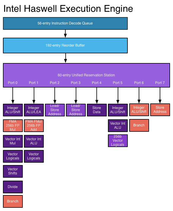