
The objective of this study was to train a network that can identify species of British freshwater fish on RGB images. The image may contain anything (people, animals etc.) providing there is only one species of fish present. No set accuracy was defined for success, rather the study aims to understand what can be achieved with limited data and the best approach to take in this scenario.
In total 14 different species of British freshwater fish were selected, with 100 images for each class collected using the google_images_download library. Manual QC of this dataset was undertaken to remove any anomalous results returned by the library which were not representative of a given class e.g. images containing multiple different species of fish. The number of samples remaining after this QC per class can be found in figure 1. Raw data and labels can be downloaded here.
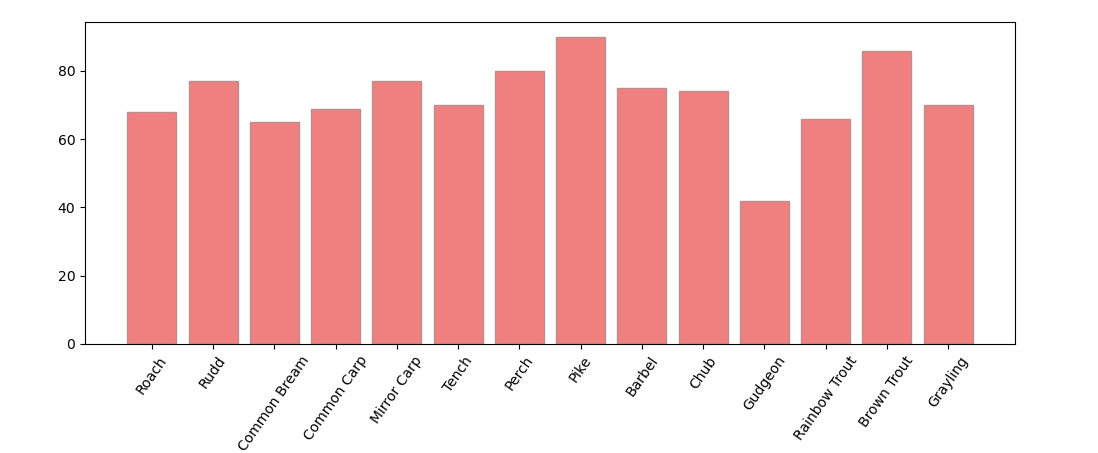
Figure 1. Number of samples per class present in the entire dataset.
An example of a selection of images in a single batch can be seen in figure 2, standardised with a common resolution of 222 * 222 pixels. Depending on model architecture, in some cases it was necessary to further reduce the resolution of the images in a bid to reduce model complexity and number of trainable parameters.
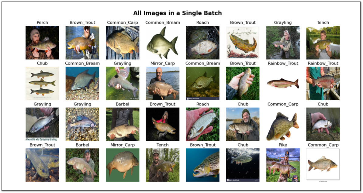
Figure 2. Example of images present in a single 32 image batch for training.
In order to achieve the project aims, numerous models of increasing complexity were trained, starting with a basic MLP before training CNN with data augmentation and transfer learning.
To begin with the most basic approach was taken, training a simple multilayer perceptron. Images were resampled to 32 * 32 with a single black-white channel, before being vectorised ready for input into the model. A small image size was chosen in an attempt to reduce the number of trainable parameters. Identifying fish species with the human eye at this resolution is difficult, but not impossible, in most cases a reasonable guess could be made. Model architecture, including the vectorisation stage can be seen in figure 3.
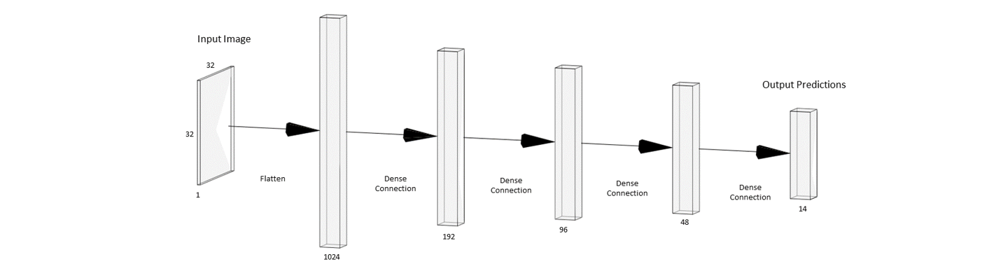
Figure 3. Simple MLP architecture formed of 4 fully connected dense layers, all with a relu activation function except the output layer which has a softmax activation.
Training was completed in batch sizes of 32, using categorical crossentropy and an adam optimiser. The results can be studied in figure 4. Accuracy peaks at around 8% which as expected is very poor, only narrowly beating a random guess.
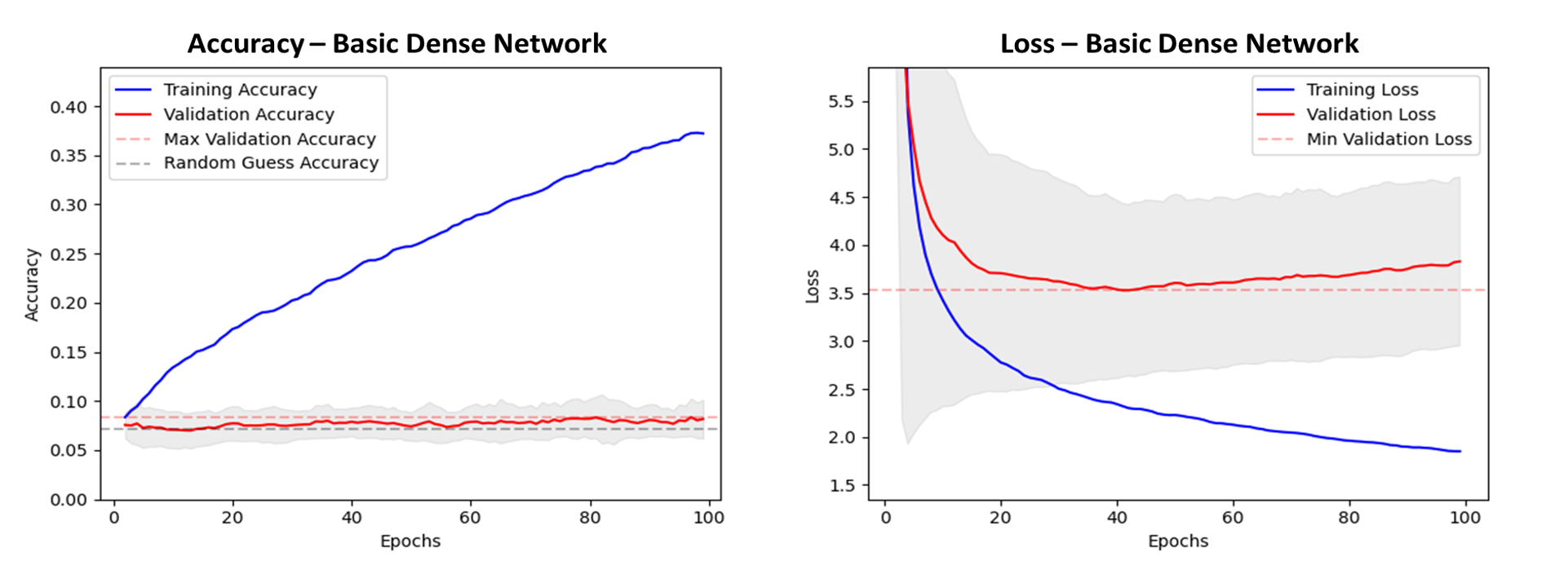
Figure 4. Accuracy and loss plots, with results averaged from 10 models trained with random weights initialisation. Grey shade shows one standard deviation. Validation accuracy suggests the model performs only marginally better than a random guess. Overfitting of the loss function on the validation data appears after around 40 epochs.
A simple and relatively shallow convnet was tested next, the architecture of which can be studied in figure 5.
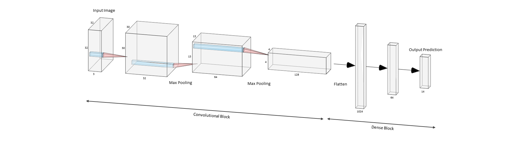
Figure 5. Three convolutional layers and two max pooling layers form the basis of the convolutional block. This is then flattened and connected to 2 dense layers for classification. All convolutional filters are 3 * 3 with a relu activation function.
To reduce the overfitting in this model, L2 regularisation was added to the loss function, and a modest dropout layer (rate = 0.2) added to the model after flattening. This resulted in a decrease in overfitting seen in the validation loss, whilst retaining the same validation accuracy when compared to with models trained without regularisation. Images were also resampled to higher resolutions for training however, the original 32 * 32 resulted in the highest accuracy. This is likely because the network is too shallow 'see' enough of the image when resolution is increased. With this configuration we see accuracy peak at 22% as seen in figure 6.
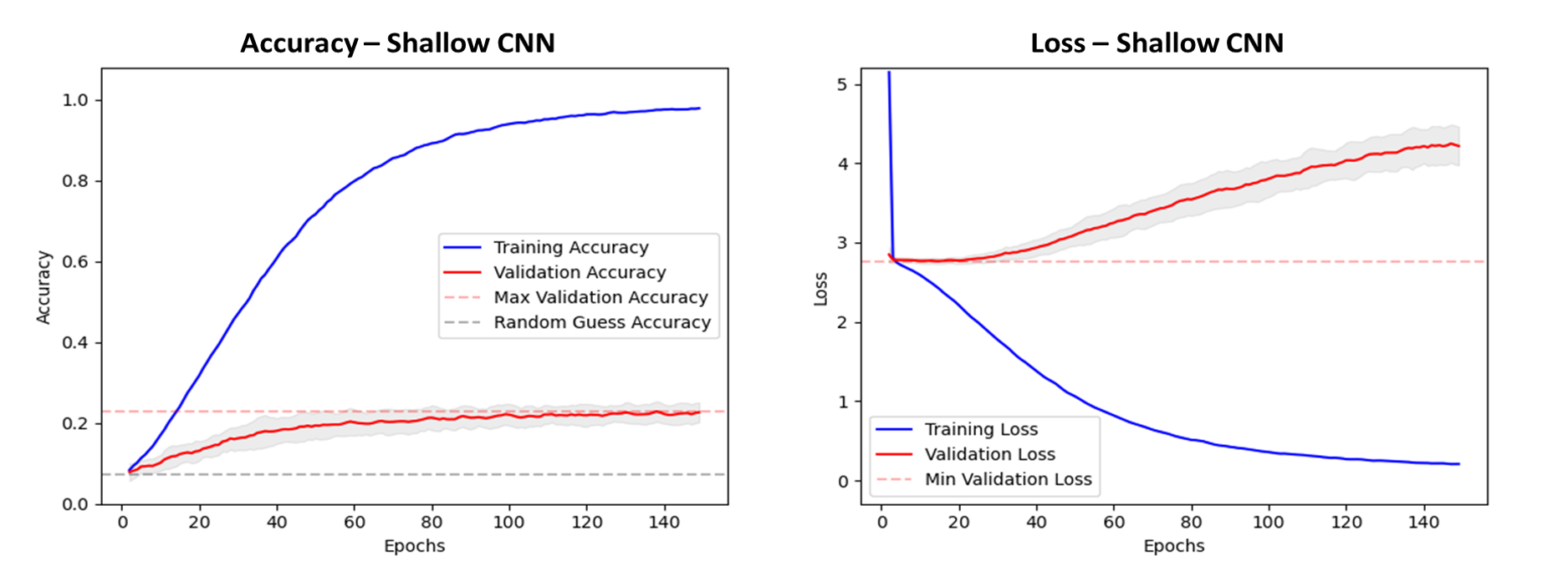
Figure 6. Accuracy and loss plots, with results averaged from 10 models trained with random weights initialisation. Grey shade shows one standard deviation. Validation accuracy rises to 22% after 90 epochs. Overfitting of the loss function on the validation data appears after around 30 epochs.
Given the conclusions of the previous model build, a deeper network was tested next, the architecture of which can be studied in figure 7.
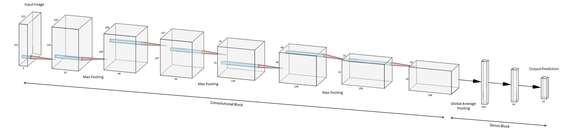
Figure 7. Seven convolutional layers and three max pooling layers form the basis of the convolutional block. This is then flattened using a global average pooling layer and connected to 2 dense layers for classification. All convolutional filters are 3 * 3 with a relu activation function.
Increasing the depth of the model allowed the image size to be increased to 222 * 222 for training. This results in a significant increase in model performance, with accuracy approximately doubling to 42%.
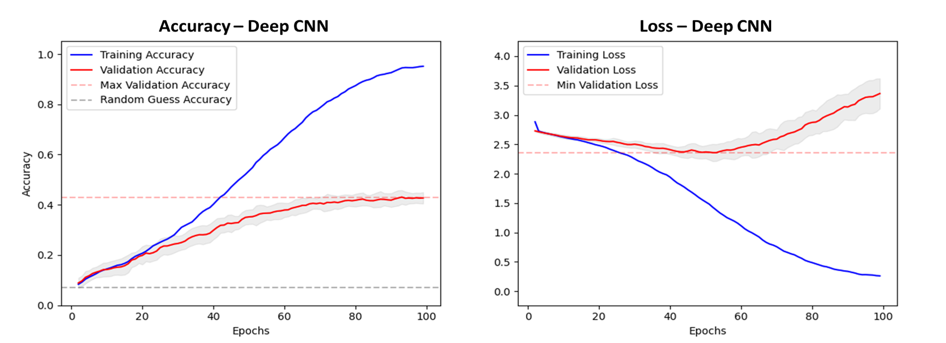
Figure 8. Accuracy and loss plots, with results averaged from 10 models trained with random weights initialisation. Grey shade shows one standard deviation. Validation accuracy rises to 42% after 100 epochs. Overfitting of the loss function on the validation data appears after around 50 epochs.
The next step taken to improve model performance was through introducing data augmentation to the training dataset. When a batch is being 'assembled' ready for training, each image has been allowed to rotate, shift position, zoom, shear and or flip. In each epoch the model is exposed to a different version of every image used in training, helping the model to generalise better and prevent overfitting. Therefore, the model will be better equipped to identify fish species irrespective of the relative size or rotation of the target. An example of data augmentation on a single training image can be seen in figure 9.
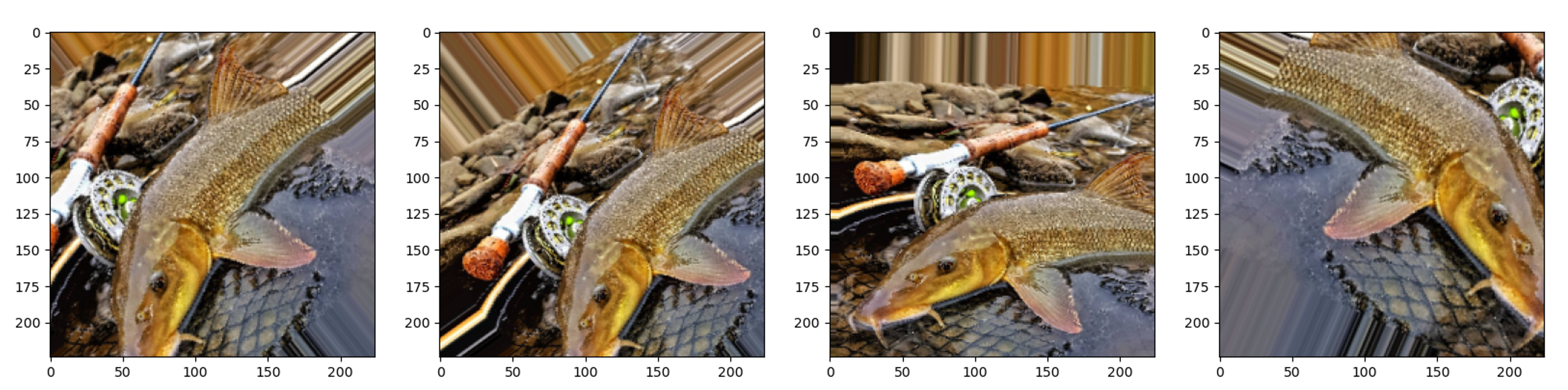
Figure 9. Data augmentation on a single image at the resolution used for training (222 * 222).
The architecture of the model has remained the same as the previous. The introduction of data augmentation alone produces a sizeable increase in accuracy to 55%, seen in figure 10.
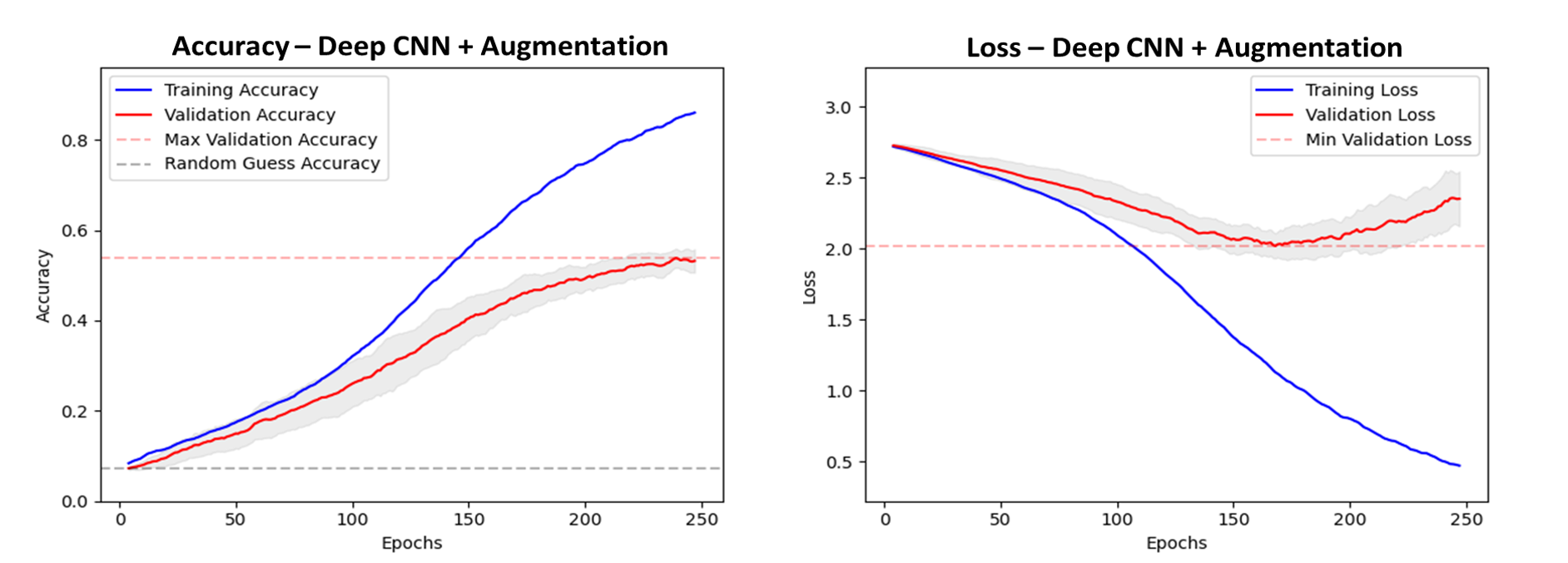
Figure 10. Accuracy and loss plots, with results averaged from 10 models trained with random weights initialisation. Grey shade shows one standard deviation. Validation accuracy rises to 55% after 240 epochs. Overfitting of the loss function on the validation data appears after around 170 epochs.
Next, an alternative approach is taken using transfer learning. In this architecture, a pre-trained convolutional base has been connected to a flatten, dropout and two trainable dense layers for classification. Various different pretrained networks available through keras were tested as the base, with xception chosen due to high model performance. As before, several input resolutions were tested, with the default image size for this base (299 * 299) selected. Using this configuration, we see a good increase in validation accuracy compared to the previous model, a rise to 72% as seen in figure 11. The untrainable convolutional base likely generalises well to the problem of fish identification due to similarities in the classes of the imagenet database which it was trained on, which already contains several classes of saltwater fish.
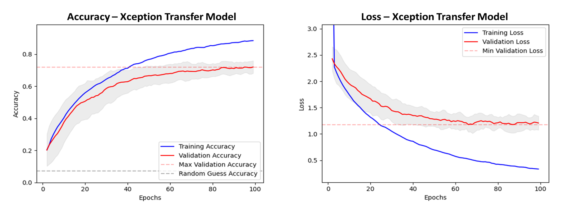
Figure 11. Accuracy and loss plots, with results averaged from 10 models trained with random weights initialisation. Grey shade shows one standard deviation. Validation accuracy rises to 72% after 100 epochs. We see no inflection in the validation loss, suggesting we have little or no overfitting.
This project is licensed under the MIT License. See the LICENSE file for details.