quentin-dev937 / glass-project

Data science project about glass classification. The goal is to classify 214 glass into 6 categories, based on their chemical composition

Glass Project

The goal of this project is to perform the classification of glass materials based on their chemical composition. This dataset was download from the Kaggle website: https://www.kaggle.com/datasets/uciml/glass

Original source: https://archive.ics.uci.edu/ml/datasets/Glass+Identification

Dataset

This dataset is quite small. As we can observe, only 214 obervations (lines) and 10 variables (columns) are at our disposal.

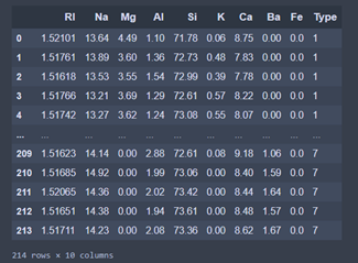
There is 9 predictive variables (features) and 1 target variable. The predictive variables are used to predict the target variable

Predictive variables

• RI: Refraction index of the glass.
• Na, Mg, Al, Si, K, Ca, Ba, Fe: weight percent in corresponding oxide used to synthetize the glass.

Target variable

• Type: the type of glass which can be one of 6 categories represented by an integer in the dataset (correspondance below).

1: Building Window (processed)

2: Building Window (non processed)

3: Vehicule Window (processed)

5: Container

6: Tableware

7: Headlamp

Data Analysis

Data types and Missing values

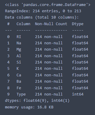
The variables are of two types: float (continues values) and integer (discrete values) and no values are missing.

Data statistical description

Some of the variables are skewed (Mg oxyde) and others are well centered (Si oxyde). Indeed, the mean and the median are quite different for the Mg variable but are very similar for the Si variable. Also, the standard deviations is high for the Mg variable and low for the Si variable.

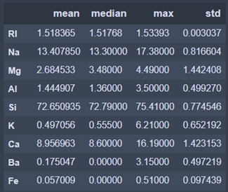
We can add that the variables don't have the same scale.

• We can observe that the weighted percentage of the Si oxyde is way higher than the other oxyde. This is explained by the fact that glass are mostly made of Si oxyde.

Data correlation

The analysis of the data correlation is a good way to detect redundant features that can be discard. In our case, we looked at the spearman correlation between features only (the target variable is categorical).

The next figure report the absolute value of the spearman correlation for each predictive variable with the other.

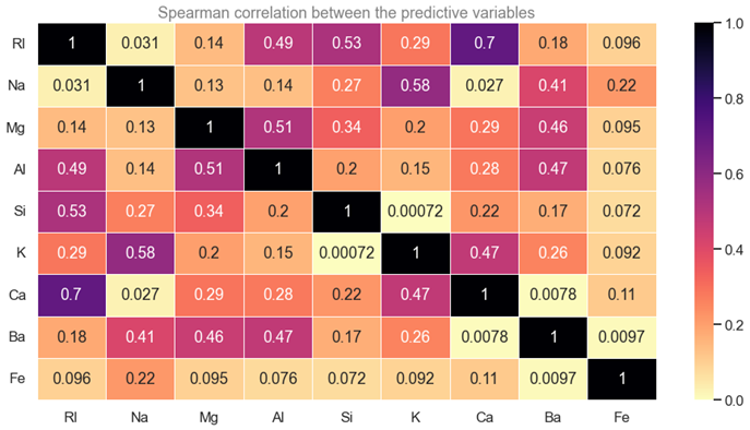
The most correlated variables are the Ca oxyde and the reflective index (0.7). So the refractive index and the weighted percentage of Ca oxyde evolve together. The features are not sufficiently correlated (< 0.9) to be discard so we keep them all.

Target modes

As mentioned before, there are 6 categories of glass in the target variable. The graphique below displays the proportion of each categories.

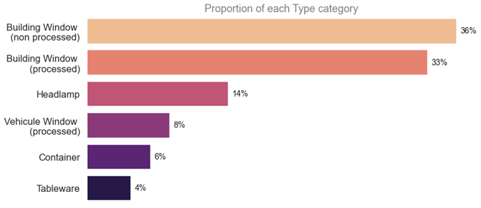
As we can observe, the categories are highly unbalanced with 36% of the data belonging to the "Building Window (non processed)" category and 4% of the data belonging to the "Tableware" category.

Now, it's time to apply data science algorithm to our data. We can recall that the target variable is very unbalanced and the predictive variables don't have the same scale nor the same range. Furthermore, the number of observations in the dataset is very low. So, an additonal phase of data processing is needed to make the data more suitable for our algorithm.

But first, the dataset is divided into 2 parts: one for the training (80%: 171 values) and one for the validation (20%: 43 values).

Data processing

Scaling

The first steps of the processing phase is the scaling of the data in order to have them at the same scale. Since some predictive variables are also skewed, the robust version of the Standard scaler is used.

Adding training observations

In order to optimize the training of the algorithm and to obtain a more balanced training set, we used the Random over Sampling method to add data to the training set.

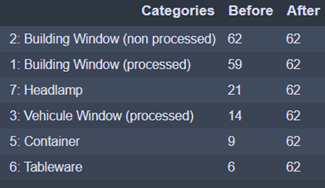
In this way, no category is disavantaged.

The next step: the modelisation

Data modelisation

Algorithm

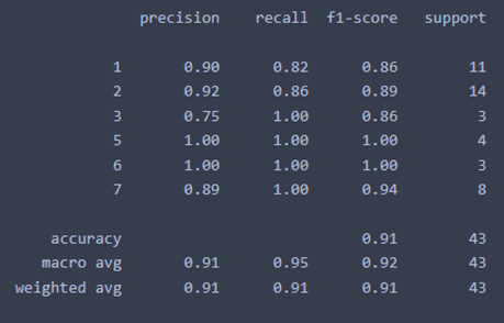
We used a simple but quite efficient Machine Learning algorithm to perform the task of data modelisation: the Random Forest Classifier without modifying the initial parameters.

Results

This algorithm reached 91% accuracy on the validation set which is good.

The confusion matrix allow us to better understand the performance of the model on the validation set. This graphic show the number of values for each real and predicted category.

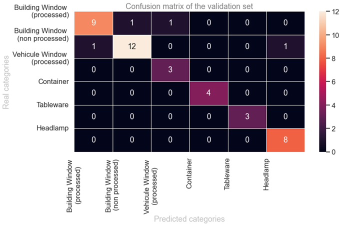
Most of the categories are well predicted as most of the values are located in the diagonal. Every values not located in the diagonal are errors of prediction fo the algorithm. Among the 43 observations in the validation set, only 4 have been misclassified.

Model Interpretation

The last step is the interpretation of the model. Basically, the goal is to get answer to those questions:

• Which predictive variables are important (and which are not so important) ?
• How are they impacting the model ?

We used the SHAP tools to create a graph to answer those questions.

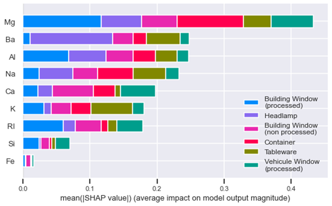
The graphic show the variables (features) inportance of the model. The Mg oxyde is the most important feature and the Fe oxyde is the least important feature. But every features add an impact on the model decision.

The other interesting aspect is how each feature is connected to a category of glass. For exemple:

• Mg oxyde is important to the "Building window processed" category
• Ba oxyde is important to the "Headlamp" category but is almost uninportant for "Building window processed" category
• K oxyde is important to the "Tableware" category.

Conclusion

This dataset is quite fun and very approchable to analyse. This short study aimed to display a wide range of tools of data science like scaling, resampling, data vizualisation, modelling and model interpretation.

As a perspective, it could be interesting to:

• have more data.
• train differents models.
• perform cross validation (training and testing on differents subset of the data).