LunarTech Academy Get Started

- Refreshment - Real Numbers and Vector Space
- Refreshment - Norm of Vector
- Refreshment - Cartesian Coordinate System & Unit Circle
- Refreshment - Angles, Unit Circle and Triogonmetry
- Refreshment - Norm vs Euclidean Distance
- Refreshment - Pythagorean Theorem & Orthogonality
- Why these pre-requisits matter
- Module 1: Foundations of Vectors
- Module 2: Special Vectors and Operations
- Module 3: Advanced Vector Concepts
- Module 4: Dot Product, Cauchy-Schwarz and Its Applications
- Module 1: Foundations of Linear Systems & Matrices
- Module 2: Introduction to Matrices
- Module 3: Core Matrix Operations
- Module 4: Solving Linear Systems - Gaussian Reduction, REF, RREF
- Module 5: Advanced Matrix Concepts and Operations - Laws, Transpose, Inverses
- Module 1: Algebraic Laws for Matrices
- Module 2: Determinants and Their Properties
- Module 3: Matrix Inverses (2x2, 3x3) and Identity Matrix
- Module 4: Transpose of Matrices: Properties and Applications
- Module 1: Vector Spaces, Projections and Gram-Schmidt Process
- Module 2: Special Matrices and Their Properties
- Module 3: Introduction to Matrix Factorization and Applications
- Module 4: QR Decomposition
- Module 5: Eigenvalues, Eigenvectors, and Eigen Decomposition
- Module 6: Singular Value Decomposition (SVD) and Its Applications

Check out Fundamentals Of Statistics For Data Scientists and Data Analysts blog post in Towards Data Science
Required Files:
- Multiple Linear Regression OLS Python Code
- Multiple Linear Regression OLS Diabetes Data Example Python Code
- Multiple Linear Regression OLS Boston Data Example Python Code
- Multiple Linear Regression OLS Boston Data Output
- Multiple Linear Regression OLS Boston Data Output 2
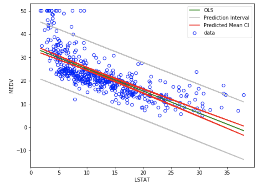
Linear regression is a linear approach to model the relationship between a scalar response (dependent varaible) and one or more explanatory variables (independent variables). The case of having single explanatory variable, the method is referred as simple linear regression. In case of having multiple explanatory variablea, the method is referred as multiple linear regression. Ordinary least squares (OLS) is a type of linear least squares method for estimating the unknown parameters in a linear regression model. OLS chooses the parameters of a linear function of a set of explanatory variables by using the principle of least squares that minimizes the sum of the squares of the residuals" (differences between the observed dependent variable and those predicted by the linear function). The method is largely applied in Econometrics, Finance, Data Science and other subject areas.

- Kumari, K. and Yadav, S. (2018). Linear regression analysis study. 4101(4), 33
- Kaya, U., Neşe, G. (2013). A Study on Multiple Linear Regression Analysis. 1016(106), 234–240
Supporting Files:
LDA in Machine Learning

Linear discriminant analysis (LDA) (don't confuss this with Latent Dirichlit Allocation which is Topic Modelling technique) is a generalization of Fisher's linear discriminant, which is a statistical method to find a linear combination of features that characterizes/separates two or more classes of objects. The resulting combination may be used as a linear classifier. LDA is closely related to analysis of variance (ANOVA) and regression analysis, which also attempt to express one (dependent) variable as a linear combination of other (independent) variables. However, ANOVA uses a continuous dependent variable and categorical independent variables, whereas LDA uses a categorical dependent variable (classes of LDA) and continuous independent variables.
Logistic regression and Probit regression are more similar to LDA than ANOVA is, as they also explain a categorical (dependent) variable by the values of continuous (independent) variables. The key difference between Logistic Regression/Probit regression and LDA is the assumption about the probability distribution about the explanatory (independent) variables. In case of LDA , fundamental assumtion is that the independent variables are normally distributed. This can be checked by looking at the probability distribution of the variables. Note: the code contains LDA and robust LDA mannually written functions (checked with the library function's output)
Publications:
- Nasar, S., Aldian, A., Nuredin, J., and Abusaeeda, I. (2016). Classification depend on linear discriminant analysis using desired outputs. 1109(10)
- Zhao, H., Wang, Z., and Nie, F. (2019) A New Formulation of Linear Discriminant Analysis for Robust Dimensionality Reduction. 31(4), 629-640,
Supporting Files:
Kolmogorov–Smirnov test (K–S test or KS test) is a nonparametric test of the equality of continuous, one-dimensional probability distributions that can be used to compare a sample with a reference probability distribution (one-sample K–S test), or to compare two samples (two-sample K–S test). The KS statistic quantifies a distance between the empirical distribution function of the sample and the cumulative distribution function of the reference distribution, or between the empirical distribution functions of two samples. In this case it has been calculated using Garch distribution. The null distribution of this statistic is calculated under the null hypothesis that the sample is drawn from the reference distribution (in the one-sample case) or that the samples are drawn from the same distribution (in the two-sample case).
Publications:
- Richard S. & Pierre L. (2011), "Computing the Two-Sided Kolmogorov-Smirnov Distribution," Journal of Statistical Software, 39, 1-18.
Supporting Files:
k-Nearest Neighbour Imputation techique is one of the most popular imputation techniques to handle missing data which can cause problems in many machine learning algorithms. Missing values exist in almost all datasets and it is essential to handle them properly in order to construct reliable machine learning models with optimal statistical power. This imputer utilizes the k-Nearest Neighbors method to replace the missing values in the datasets with the mean value from the parameter ‘n_neighbors’ nearest neighbors found in the training set. By default, it uses a Euclidean distance metric to impute the missing values. One thing to be aware of here is that the kNN Imputer does not recognize text data values. Using strings instead of numerical data values will result in errors. To solve this, one can use One-Hot-Encoder to transform string type varaibles to numerical ones. Another important point here is that the kNN Imptuer is a distance-based imputation method and it requires normalized data.
Publications:
- Pan, R. (2015). "Missing data imputation by K nearest neighbours based on grey relational structure and mutual information," The International Journal of Artificial Intelligence, Neural Networks, and Complex Problem-Solving Technologies, 42(4).
Supporting Files:
Case Study that aims to find the rankings of the cities in United States based on a single combination of 9 rating variables using multivariate techniques: Principal Components Analysis (PCA) and Factor Analysis (FA). Moreover, we will also use Canonical Correlation Analysis (CCA) to get more insight of this data and investigate the correlation between two sets of rating variables (if existing). We aim to find the linear combination of rating variables that would maximally explain the variation of the data and rank the U.S. cities according to this new rating criterion.
Supporting Files:
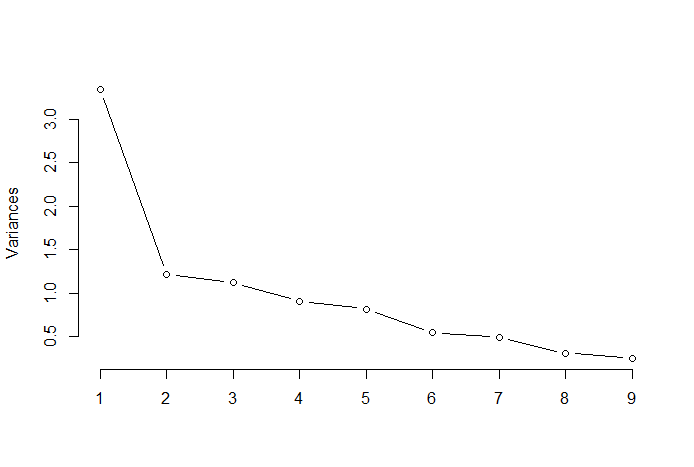
PCA is used in exploratory data analysis and for making predictive models. It is commonly used for dimensionality reduction by projecting each data point onto only the first few principal components to obtain lower-dimensional data while explaining as much possible variation in the data. PCA is scale-insensitive, therefore data normalization is not necessary. The first principal component can equivalently be defined as a direction that maximizes the variance of the projected data. The principal components are eigenvectors of the data's covariance matrix. To determine optimal number of PC's one can use one of the following methods: Keizer Rule, Elbow Rule
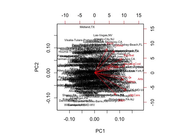
Principal Component Analysis (PCA) Application Example
Biplot with scaled data where yoou can observe that Crime and Education have the smallest margins and the remaining variables show substantial variations. First three principal components explain 63.10% of the total variation in data. Applying the ”elbow rule” it can be seen that one can optimally retain 3 components.
Publicatioons:
- Mishra, S., Sarkar, U., Taraphder, S. (2017). "Principal Component Analysis". International Journal of Livestock Research. 1(10)
Supporting Files:
Factor analysis is another statistical method for dimensionality reduction. It is one of the most commonly used inter-dependency techniques and is used when the relevant set of variables shows a systematic inter-dependence and the objective is to find out the latent factors that create a commonality. So, the model attempts to explain a set of p observations in each of n individuals with a set of k common factors (F) where there are fewer factors per unit than observations per unit (k<p). In factor analysis the factors are calculated to maximize between-group variance while minimizing in-group variance. They are factors because they group the underlying variables. Unlike the PCA, in case of FA the data needs to be normalized if needed, given the FA assumtion that the data follows normal distribution.
Publications:
- Cattell, R. (1965). A Biometrics Invited Paper. Factor Analysis: An Introduction to Essentials I. The Purpose and Underlying Models. Biometrics, 21(1), 190-215
Supporting Files:
Canonical Correlation analysis is the analysis of multiple-X multiple-Y correlation. The Canonical Correlation Coefficient measures the strength of association between two Canonical Variates. Canonical Variants are not factors because only the first pair of canonical variants groups the variables in such way that the correlation between them is maximized. The second pair is constructed out of the residuals of the first pair in order to maximize correlation between them. Therefore the canonical variants cannot be interpreted in the same way as factors in factor analysis. Also the calculated canonical variates are automatically orthogonal, i.e., they are independent from each other.
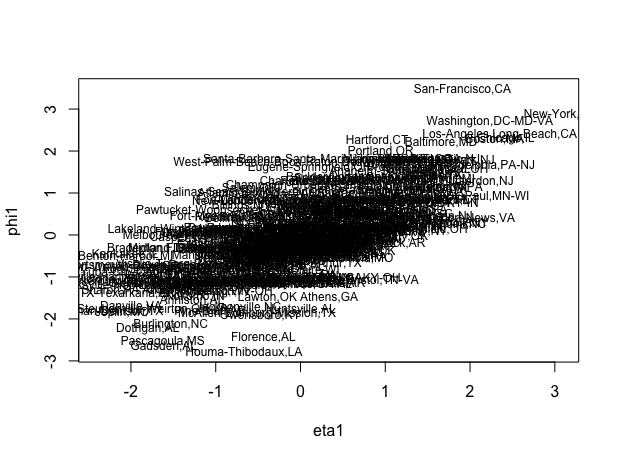
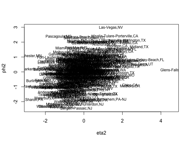
Canonical Correlation Analysis (CCA) Application Example
Figures showing clear correlation between X and Y scores for the first canonical correlation which is not the case for the second factor, where one can observe some correlation but not significant. This shows that the first canonical correlation is important but second one is not.
Publications: - Yang, X., Weifeng, L., Liu W., and Tao, D., (2019) "A Survey on Canonical Correlation Analysis," in IEEE Transactions on Knowledge and Data Engineering, 10(1109)
Supporting Files:
FastMCD statistical algorithm to estimate scaltter and location parameters FASTMCD computes the MCD estimator of a multivariate data set. This estimator is given by the subset of h observations with smallest covariance determinant. The MCD location estimate is then the mean of those h points,and the MCD scatter estimate is their covariance matrix. The default value of h is roughly 0.75n (where n is the total number of observations), but the user may choose each value between n/2 and n.
The MCD method is intended for continuous variables, and assumes that the number of observations n is at least 5 times the number of variables p. If p is too large relative to n, it would be better to first reduce p by variable selection or principal components. It is a robust method in the sense that the estimates are not unduly influenced by outliers in the data, even if there are many outliers. Due to the MCD's robustness, we can detect outliers by their large robust distances. The latter are defined like the usual Mahalanobis distance, but based on the MCD location estimate and scatter matrix (instead of the nonrobust sample mean and covariance matrix).
The FASTMCD algorithm uses several time-saving techniques which make it available as a routine tool to analyze data sets with large n,and to detect deviating substructures in them. A full description of the algorithm can be found in: An important feature of the FASTMCD algorithm is that it allows for exact fit situations, i.e. when more than h observations lie on a (hyper)plane. Then the program still yields the MCD location and scatter matrix, the latter being singular (as it should be), as well as the equation of the hyperplane.
Publications:
- Rousseeuw, P.J. (1984), "Least Median of Squares Regression," Journal of the American Statistical Association, 79, 871-881
- Rousseeuw, P.J. and Van Driessen, K. (1999), "A Fast Algorithm for the Minimum Covariance Determinant Estimator," Technometrics, 41, 212-223
Supporting Files:
Missing data is a widely-known issue in numerous fields of scientific research mainly because most of the statistical methods require complete data. Missing values in the data can have different reasons: respondents can mistakenly skip question resulting in nonresponse,the data might be combined from different surveys leading to incomplete information, failure in the net- work leading to the loss in the data and sometimes individuals consciously skip some questions which they might have found too personal, embarrassing or they simply didn’t want to share that information. Especially when dealing with large data sets,very often observations that con- tain missing values are being simply removed from research to get complete data and perform the analysis. This might lead to biased results with lower statistical power. Therefore, it is important to know the reason for missingness in the data and it’s effect on the analysis. This Case Study about missing data detection, known missing data menchanism, missing data imputation techniques and its application in Linear Regression and robus MM regression analysis.
- Missing data detection
- Missing data mechanisms (MNAR, MCAR, MAR)
- Missing data imputation techniques (Single Imputation, Multiple Imputation)
- OLS regression
- Robust MM regression
Supporting Files:
Finite mixture distributions are a weighted average of a finite number of distributions. The latter are usually called the mixture components. The weights are usually described by a multinomial distribution and are sometimes called mixing proportions. The mixture components may be the same type of distributions with different parameter values but they may also be completely different distributions Therefore, finite mixture distributions are very flexible for modeling data. They are frequently used as a building block within many modern econometric models. This model is especifially helpful when segmenting customers into segments while taking into account that customers aree different: heterogenous.
Publications:
- Melnykov, V.and Maitra, R., (2010). "Finite mixture models and model-based", in Associate Editor for the IMS, 4, 80–116


