ziwei-utc / bhrm

R package for Bayesian Hierarchical Richards Model

BHRM: An R package implementing Bayesian Hierarchical Richards Model to Estimate Infection Trajectories and Identify Risk Factors for the COVID-19 Outbreak

Contents

• Overview
• Installation
• BHRM
• Example
• References

Overview

An R package BHRM of the paper titled "Estimation of COVID-19 spread curves integrating global data and borrowing information", PLOS ONE, (2020) is available here. This is a joint project of Ph.D. student Bowen Lei ([email protected]), and a former Ph.D. student Dr. Se Yoon Lee ([email protected]), and a University Distinguished Professor Dr. Bani K. Mallick ([email protected]) at Texas A&M University.

The objective of the R package BHRM is implement Bayesian Hierarchical Richards Model (BHRM) applied to the COVID-19 dataset obtained from multiple countries. BHRM is an all-in-one R package that includes dataset, Gibbs sampling algorithm, and visualization tools from output.

The sources of the datasets are:

1. Center for Systems Science and Engineering at Johns Hopkins University
2. World Bank
3. World Health Organization
4. National Oceanic and Atmospheric Administration

Required R version

R version 4.0.4 (or higher)

Installation

require(devtools)
devtools::install_github("StevenBoys/BHRM", ref = "HEAD")
library(BHRM)

BHRM

Bayesian hierarchical Richards model (BHRM) is a fully Bayesian version of non-linear mixed effect model where (i) on the first stage infection trajectories from N subjects (subjects can be states in a country, countries, etc) are described by the Richards growth curve, and (ii) on the second stage the sparse horseshoe prior indentifies important predictors that largely affect on the shape the curve. Richards growth curve has been widely used to describe epidemiology for real-time prediction of outbreak of diseases. Refer to our paper "Estimation of COVID-19 spread curves integrating global data and borrowing information", PLOS ONE, (2020) for a detailed explanation of the BHRM.

Figure 1 shows (i) a hierarchy of the BHRM (top panel) and (ii) its directed asymetric graphical model representation (bottom panel)

Figure 1: A hierarhcy of the Bayesian Hierarchical Richards Model (top) and its graphical model representation (bottom).

Example

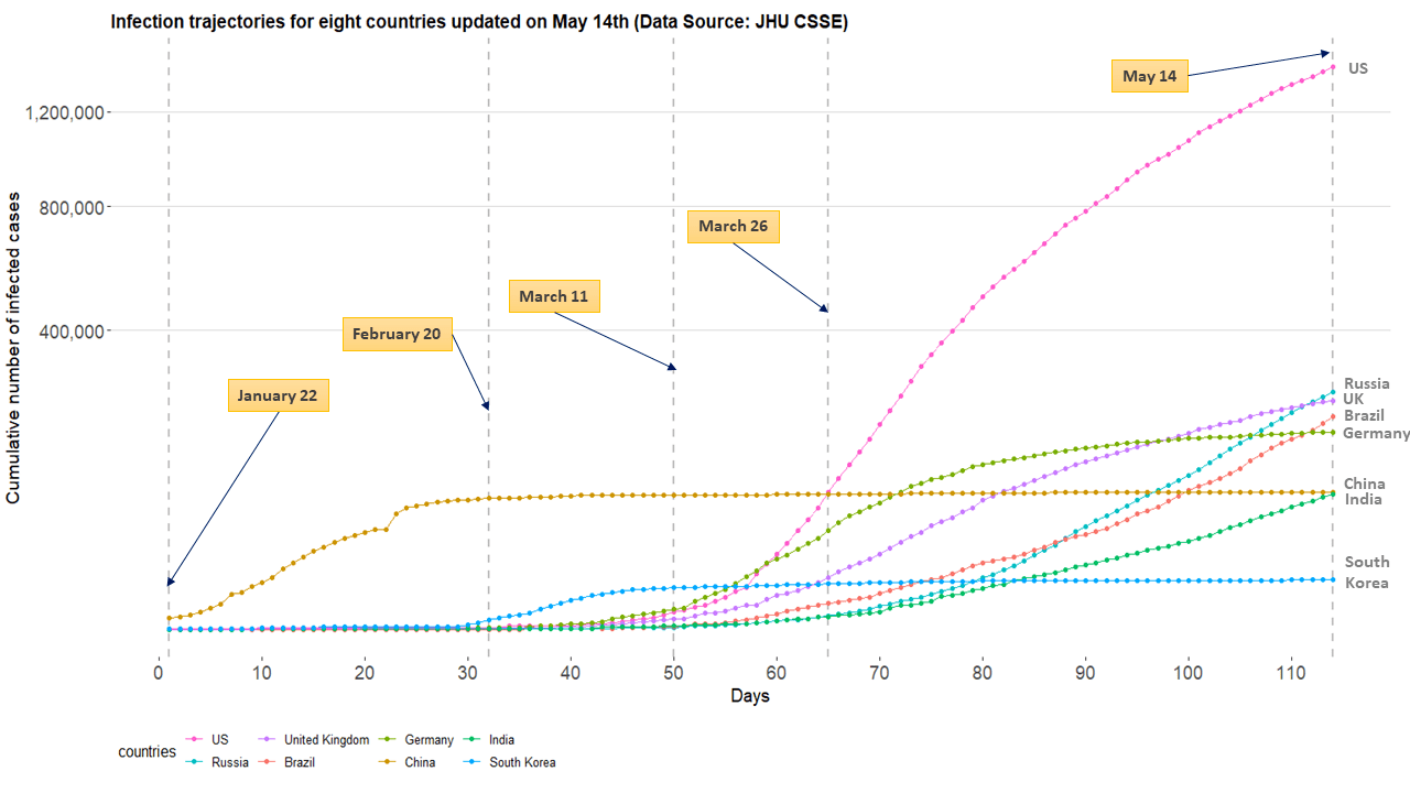
R package BHRM contains COVID-19 dataset comprises (i) time_series_data and (ii) design_matrix to train the BHRM. time_series_data includes infection growth curve from January 22nd to May 14th for 40 global countries and design_matrix has 45 predictors that cover health care resources, population statistics, disease prevalence, etc. Figure 2 displays infection trajectories for eight countries (US, Russia, UK, Brazil, Germany, China, India, and South Korea), spanning from January 22nd to May 14th, which accounts for 114 days.

Figure 2: Infection trajectories for eight countries updated on May 14th (Data source: JHU CSSE).

To load the COVID-19 dataset, use

library(BHRM)
# load the data
data("design_matrix")
data("time_series_data")
Y = time_series_data[, -c(1:2)]; X = design_matrix[, -c(1:2)]

To train BHRM with the aforementioned dataset, use the R function BHRM_cov as following way. The BHRM_cov implements a Gibbs sampling algorithm to sample from the posterior distribution for the BHRM given the dataset. It may need at least 10 minutes to train the data, depending on CPU speed.

# set the hyperparameters
seed.no = 1 ; burn = 5000 ; nmc = 5000 ; thin = 30; varrho = 0
pro.var.theta.2 = 0.0002 ; pro.var.theta.3 = 0.05; mu = 0 ; rho.sq = 1
t.values = list(); num_days = 14
for(i in 1:nrow(Y)){
  t.values[[i]] = c(1:(ncol(Y) - num_days))
}
Y = Y[, c(1:(ncol(Y) - num_days))]
# run the model
res_cov = BHRM_cov(Y = Y, X = X, t.values = t.values, seed.no = seed.no, burn = burn,   
                   nmc = nmc, thin = thin, varrho = varrho, pro.var.theta.2 = pro.var.theta.2, 
                   pro.var.theta.3 = pro.var.theta.3, mu = mu, rho.sq = rho.sq)  

To visualize the training results, use R functions extrapolate and plot_RM as follows

# make extrapolations
extra_list = extrapolate(res_cov, Y, 1)
# make a plot to see the performance of the extrapolations
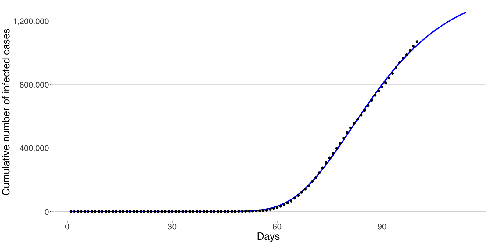
plot_RM(extra_list$mean, Y[1, ], y_name = "Cumulative number of infected cases")

Figure 3: Comparison between the real trajectory and extrapolated values.

We can also compute flat points of the estimated Richards curve by using R function flat_time_point. As shown in the Figure 5, the vertical blue lines refer to the three flat time points, while the horizontal blue line corresponds to the final epidemic size.

out = flat_time_point(res_cov, Y, 1, y_name = "Cumulative number of infected cases")
out$figure

Figure 4: Plot that shows flat time points in the trajectory.

To obtain the values of flat time points and epidemic size, use

out$flat_time_points
# [1] 228.5129 191.7026 154.8270
out$epi_size
# [1] 1428479

We can use R function var_sele to visualize the result of covartiates analysis obtained via sparse horseshoe prior. Figure 5 displays 95% posterior credible intervals for each of the three coefficient vectors used in the second stage of the BHRM.

# check the important factors for beta1
var_selection1 = var_sele(beta.vec = res_cov$thinned.beta.1.vec, j = 1)
# check the important factors for beta2
var_selection2 = var_sele(beta.vec = res_cov$thinned.beta.2.vec, j = 2)
# check the important factors for beta3
var_selection3 = var_sele(beta.vec = res_cov$thinned.beta.3.vec, j = 3)

# check the names of the top covariates selected
var_selection1$id_sele
# [1] 40 41 32 19 37 27  5 30 18 12
var_selection2$id_sele
# [1] 13 20 40 36 33 37  1 21 31  7
var_selection3$id_sele
# [1] 40  2 26 33 44  7 41 30 18  5

# plot the figure for 95% credible interval of each covariates
var_selection1$figure
var_selection2$figure
var_selection3$figure

Figure 5: 95% confidence intervals of the 20 potential factors for beta1 (top), beta2 (middle), and beta3 (bottom).

Table 1 summarizes results of the panels in Figure 5.

Table 1: Significant covariates explaining the curve parameters of the Richards curve.

References

[1] Se Yoon Lee, Bowen Lei, and Bani K. Mallick. (2020) “Estimation of COVID19 spread curves integrating global data and borrowing information,” PLOS ONE

[2] Se Yoon Lee and Bani K. Mallick. (2021) “Bayesian Hierarchical modeling: application towards production results in the Eagle Ford Shale of South Texas,” Sankhyā: The Indian Journal of Statistics, Series B ; [Github]

[3] Davidian, M., and Giltinan, D. M. (1995). Nonlinear models for repeated measurement data (Vol. 62). CRC press.