GithubHelp home page GithubHelp logo

fasiha / ebisu Goto Github PK

View Code? Open in Web Editor NEW
305.0 18.0 32.0 8.16 MB

Public-domain Python library for flashcard quiz scheduling using Bayesian statistics. (JavaScript, Java, Dart, and other ports available!)

Home Page: https://fasiha.github.io/ebisu

License: The Unlicense

Python 63.15% JavaScript 4.73% Jupyter Notebook 32.12%
spaced-repetition bayesian-statistics statistical-methods recall-probabilities review probability-density quiz recall monte-carlo python

ebisu's Introduction

Ebisu: intelligent quiz scheduling

Important links

Table of contents

Introduction

Consider a student memorizing a set of facts.

  • Which facts need reviewing?
  • How does the student’s performance on a review change the fact’s future review schedule?

Ebisu is a public-domain library that answers these two questions. It is intended to be used by software developers writing quiz apps, and provides a simple API to deal with these two aspects of scheduling quizzes:

  • predictRecall gives the current recall probability for a given fact.
  • updateRecall adjusts the belief about future recall probability given a quiz result.

Behind these two simple functions, Ebisu is using a simple yet powerful model of forgetting, a model that is founded on Bayesian statistics and exponential forgetting.

With this system, quiz applications can move away from “daily review piles” caused by less flexible scheduling algorithms. For instance, a student might have only five minutes to study today; an app using Ebisu can ensure that only the facts most in danger of being forgotten are reviewed.

Ebisu also enables apps to provide an infinite stream of quizzes for students who are cramming. Thus, Ebisu intelligently handles over-reviewing as well as under-reviewing.

This document is a literate source: it contains a detailed mathematical description of the underlying algorithm as well as source code for a Python implementation (requires Scipy and Numpy). Separate implementations in other languages are detailed below.

The next section is a Quickstart guide to setup and usage. See this if you know you want to use Ebisu in your app.

Then in the How It Works section, I contrast Ebisu to other scheduling algorithms and describe, non-technically, why you should use it.

Then there’s a long Math section that details Ebisu’s algorithm mathematically. If you like Beta-distributed random variables, conjugate priors, and marginalization, this is for you. You’ll also find the key formulas that implement predictRecall and updateRecall here.

Nerdy details in a nutshell: Ebisu begins by positing a Beta prior on recall probability at a certain time. As time passes, the recall probability decays exponentially, and Ebisu handles that nonlinearity exactly and analytically—it requires only a few Beta function evaluations to predict the current recall probability. Next, a quiz is modeled as a binomial trial whose underlying probability prior is this non-conjugate nonlinearly-transformed Beta. Ebisu approximates the non-standard posterior with a new Beta distribution by matching its mean and variance, which are also analytically tractable, and require a few evaluations of the Beta function.

Finally, the Source Code section presents the literate source of the library, including several tests to validate the math.

Quickstart

Install pip install ebisu (both Python3 and Python2 ok 🤠).

Data model For each fact in your quiz app, you store a model representing a prior distribution. This is a 3-tuple: (alpha, beta, t) and you can create a default model for all newly learned facts with ebisu.defaultModel. (As detailed in the Choice of initial model parameters section, alpha and beta define a Beta distribution on this fact’s recall probability t time units after it’s most recent review.)

Predict a fact’s current recall probability ebisu.predictRecall(prior: tuple, tnow: float) -> float where prior is this fact’s model and tnow is the current time elapsed since this fact’s most recent review. tnow may be any unit of time, as long as it is consistent with the half life’s unit of time. The value returned by predictRecall is a probability between 0 and 1.

Update a fact’s model with quiz results ebisu.updateRecall(prior: tuple, success: int, total: int, tnow: float) -> tuple where prior and tnow are as above, and where success is the number of times the student successfully exercised this memory during the current review session out of total times—this way your quiz app can review the same fact multiple times in one sitting. Bonus: you can also pass in a floating point success between 0 and 1 for soft-binary quizzes! The returned value is this fact’s new prior model—the old one can be discarded.

IPython Notebook crash course For a conversational introduction to the API in the context of a mocked quiz app, see this IPython Notebook crash course.

Further information Module docstrings in a pinch but full details plus literate source below, under Source code.

Alternative implementations Ebisu.js is a JavaScript port for browser and Node.js. ebisu-java is for Java and JVM languages. ebisu_dart is a Dart port for browser and native targets. obliviate is available for .NET.

How it works

There are many scheduling schemes, e.g.,

Many of these are inspired by Hermann Ebbinghaus’ discovery of the exponential forgetting curve, published in 1885, when he was thirty-five. He memorized random consonant–vowel–consonant trigrams (‘PED’, e.g.) and found, among other things, that his recall decayed exponentially with some time-constant.

Anki and SuperMemo use carefully-tuned mechanical rules to schedule a fact’s future review immediately after its current review. The rules can get complicated—I wrote a little field guide to Anki’s, with links to the source code—since they are optimized to minimize daily review time while maximizing retention. However, because each fact has simply a date of next review, these algorithms do not gracefully accommodate over- or under-reviewing. Even when used as prescribed, they can schedule many facts for review on one day but few on others. (I must note that all three of these issues—over-reviewing (cramming), under-reviewing, and lumpy reviews—have well-supported solutions in Anki by tweaking the rules and third-party plugins.)

Duolingo’s half-life regression explicitly models the probability of you recalling a fact as \(2^{-Δ/h}\), where Δ is the time since your last review and \(h\) is a half-life. In this model, your chances of passing a quiz after \(h\) days is 50%, which drops to 25% after \(2 h\) days. They estimate this half-life by combining your past performance and fact metadata in a large-scale machine learning technique called half-life regression (a variant of logistic regression or beta regression, more tuned to this forgetting curve). With each fact associated with a half-life, they can predict the likelihood of forgetting a fact if a quiz was given right now. The results of that quiz (for whichever fact was chosen to review) are used to update that fact’s half-life by re-running the machine learning process with the results from the latest quizzes.

The Mozer group’s algorithms also fit a hierarchical Bayesian model that links quiz performance to memory, taking into account inter-fact and inter-student variability, but the training step is again computationally-intensive.

Like Duolingo and Mozer’s approaches, Ebisu explicitly tracks the exponential forgetting curve to provide a list of facts sorted by most to least likely to be forgotten. However, Ebisu formulates the problem very differently—while memory is understood to decay exponentially, Ebisu posits a probability distribution on the half-life and uses quiz results to update its beliefs in a fully Bayesian way. These updates, while a bit more computationally-burdensome than Anki’s scheduler, are much lighter-weight than Duolingo’s industrial-strength approach.

This gives small quiz apps the same intelligent scheduling as Duolingo’s approach—real-time recall probabilities for any fact—but with immediate incorporation of quiz results, even on mobile apps.

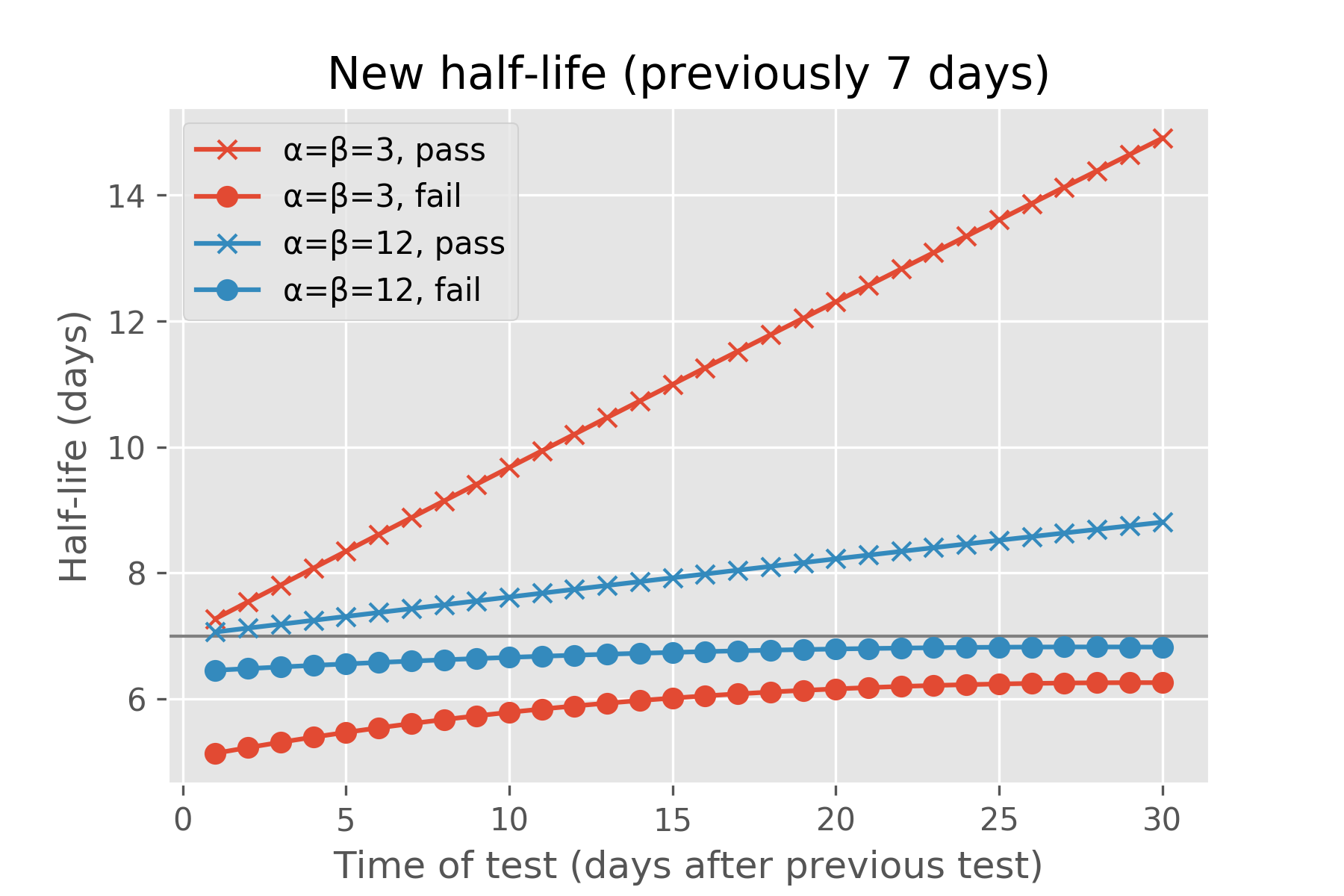
To appreciate this further, consider this example. Imagine a fact with half-life of a week: after a week we expect the recall probability to drop to 50%. However, Ebisu can entertain an infinite range of beliefs about this recall probability: it can be very uncertain that it’ll be 50% (the “α=β=3” model below), or it can be very confident in that prediction (“α=β=12” case):

figures/models.png

Under either of these models of recall probability, we can ask Ebisu what the expected half-life is after the student is quizzed on this fact a day, a week, or a month after their last review, and whether they passed or failed the quiz:

figures/halflife.png

If the student correctly answers the quiz, Ebisu expects the new half-life to be greater than a week. If the student answers correctly after just a day, the half-life rises a little bit, since we expected the student to remember this fact that soon after reviewing it. If the student surprises us by failing the quiz just a day after they last reviewed it, the projected half-life drops. The more tentative “α=β=3” model aggressively adjusts the half-life, while the more assured “α=β=12” model is more conservative in its update. (Each fact has an α and β associated with it and I explain what they mean mathematically in the next section. Also, the code for these two charts is below.)

Similarly, if the student fails the quiz after a whole month of not reviewing it, this isn’t a surprise—the half-life drops a bit from the initial half-life of a week. If she does surprise us, passing the quiz after a month of not studying it, then Ebisu boosts its expected half-life—by a lot for the “α=β=3” model, less for the “α=β=12” one.

Currently, Ebisu treats each fact as independent, very much like Ebbinghaus’ nonsense syllables: it does not understand how facts are related the way Duolingo can with its sentences. However, Ebisu can be used in combination with other techniques to accommodate extra information about relationships between facts.

The math

Bernoulli quizzes

Let’s begin with a quiz. One way or another, we’ve picked a fact to quiz the student on, \(t\) days (the units are arbitrary since \(t\) can be any positive real number) after her last quiz on it, or since she learned it for the first time.

We’ll model the results of the quiz as a Bernoulli experiment—we’ll later expand this to a binomial experiment. So for Bernoulli quizzes, \(x_t ∼ Bernoulli(p)\); \(x_t\) can be either 1 (success) with probability \(p_t\), or 0 (fail) with probability \(1-p_t\). Let’s think about \(p_t\) as the recall probability at time \(t\)—then \(x_t\) is a coin flip, with a \(p_t\)-weighted coin.

The Beta distribution happens to be the conjugate prior for the Bernoulli distribution. So if our a priori belief about \(p_t\) follow a Beta distribution, that is, if \[p_t ∼ Beta(α_t, β_t)\] for specific \(α_t\) and \(β_t\), then observing the quiz result updates our belief about the recall probability to be: \[p_t | x_t ∼ Beta(α_t + x_t, β_t + 1 - x_t).\]

Aside 0 If you see a gibberish above instead of a mathematical equation (it can be hard to tell the difference sometimes…), you’re probably reading this on GitHub instead of the main Ebisu website which has typeset all equations with MathJax. Read this document there.

Aside 1 Notice that since \(x_t\) is either 1 or 0, the updated parameters \((α + x_t, β + 1 - x_t)\) are \((α + 1, β)\) when the student correctly answered the quiz, and \((α, β + 1)\) when she answered incorrectly.

Aside 2 Even if you’re familiar with Bayesian statistics, if you’ve never worked with priors on probabilities, the meta-ness here might confuse you. What the above means is that, before we flipped our \(p_t\)-weighted coin (before we administered the quiz), we had a specific probability distribution representing the coin’s weighting \(p_t\), not just a scalar number. After we observed the result of the coin flip, we updated our belief about the coin’s weighting—it still makes total sense to talk about the probability of something happening after it happens. Said another way, since we’re being Bayesian, something actually happening doesn’t preclude us from maintaining beliefs about what could have happened.

This is totally ordinary, bread-and-butter Bayesian statistics. However, the major complication arises when the experiment took place not at time \(t\) but \(t_2\): we had a Beta prior on \(p_t\) (probability of recall at time \(t\)) but the test is administered at some other time \(t_2\).

How can we update our beliefs about the recall probability at time \(t\) to another time \(t_2\), either earlier or later than \(t\)?

Moving Beta distributions through time

Our old friend Ebbinghaus comes to our rescue. According to the exponentially-decaying forgetting curve, the probability of recall at time \(t\) is \[p_t = 2^{-t/h},\] for some notional half-life \(h\). Let \(t_2 = δ·t\). Then, \[p_{t_2} = p_{δ t} = 2^{-δt/h} = (2^{-t/h})^δ = (p_t)^δ.\] That is, to fast-forward or rewind \(p_t\) to time \(t_2\), we raise it to the \(δ = t_2 / t\) power.

Unfortunately, a Beta-distributed \(p_t\) becomes non-Beta-distributed when raised to any positive power \(δ\). For a quiz with recall probability given by \(p_t ∼ Beta(12, 12)\) for \(t\) one week after the last review (the middle histogram below), \(δ > 1\) shifts the density to the left (lower recall probability) while \(δ < 1\) does the opposite. Below shows the histogram of recall probability at the original half-life of seven days compared to that after two days (\(δ = 0.3\)) and three weeks (\(δ = 3\)). figures/pidelta.png

We could approximate this \(δ\) with a Beta random variable, but especially when over- or under-reviewing, the closest Beta fit is very poor. So let’s derive analytically the probability density function (PDF) for \(p_t^δ\). Recall the conventional way to obtain the density of a nonlinearly-transformed random variable. Since the new random variable \[p_{t_2} = g(p_t) = (p_t)^δ,\] and the inverse of this transformation is \[p_t = g^{-1}(p_{t_2}) = (p_{t_2})^{1/δ},\] the transformed (exponentiated) random variable has probability density \begin{align} P(p_{t_2}) &= P\left(g^{-1}(p_{t_2})\right) ⋅ \frac{∂}{∂p_{t_2}} g^{-1}(p_{t_2}) \\ &= Beta(p_{t_2}^{1/δ}; α, β) ⋅ \frac{p_{t_2}^{1/δ - 1}}{δ}, \end{align} since \(P(p_t) = Beta(p_t; α, β)\), the Beta density on the recall probability at time \(t\), and \(\frac{∂}{∂p_{t_2}} g^{-1}(p_{t_2})^{1/δ} = \frac{p_{t_2}^{1/δ - 1}}{δ}\). Following some algebra, the final density is \[ P(p; p_t^δ) = \frac{p^{α/δ - 1} · (1-p^{1/δ})^{β-1}}{δ · B(α, β)}, \] where \(B(α, β) = Γ(α) · Γ(β) / Γ(α + β)\) is beta function (also the normalizing denominator in the Beta density—confusing, sorry), and \(Γ(·)\) is the gamma function, a generalization of factorial. Throughout this document, I use \(P(x; X)\) to denote the density of the random variable \(X\) as a function of the algebraic variable \(x\).

Robert Kern noticed that this is a generalized Beta of the first kind, or GB1, random variable: \[p_t^δ ∼ GB1(p; 1/δ, 1, α; β)\] When \(δ=1\), that is, at exactly the half-life, recall probability is simply the initial Beta we started with.

We will use the density of \(p_t^δ\) to reach our two most important goals:

  • what’s the recall probability of a given fact right now?, and
  • how do I update my estimate of that recall probability given quiz results?

To check the above derivation in Wolfram Alpha, type in p^((a-1)/d) * (1 - p^(1/d))^(b-1) / Beta[a,b] * D[p^(1/d), y].

To check it in Sympy, copy-paste the following into the Sympy Live Shell (or save it in a file and run):

from sympy import symbols, simplify, diff
p_1, p_2, a, b, d, den = symbols('p_1 p_2 α β δ den', positive=True, real=True)
prior_t = p_1**(a - 1) * (1 - p_1)**(b - 1) / den
prior_t2 = simplify(prior_t.subs(p_1, p_2**(1 / d)) * diff(p_2**(1 / d), p_2))
prior_t2  # or
print(prior_t2)

which produces p_2**((α - δ)/δ)*(1 - p_2**(1/δ))**(β - 1)/(den*δ).

And finally, we can use Monte Carlo to generate random draws from \(p_t^δ\), for specific α, β, and δ, and comparing sample moments against the GB1's analytical moments per Wikipedia, \(E\left[(p_{t}^{δ})^N\right]=\frac{B(α + δ N, β)}{B(α, β)}\):

(α, β, δ) = 5, 4, 3
import numpy as np
from scipy.stats import beta as betarv
from scipy.special import beta as betafn
prior_t = betarv.rvs(α, β, size=100_000)
prior_t2 = prior_t**δ
Ns = np.array([1, 2, 3, 4, 5])
sampleMoments = [np.mean(prior_t2**N) for N in Ns]
analyticalMoments = betafn(α + δ * Ns, β) / betafn(α, β)
print(list(zip(sampleMoments, analyticalMoments)))

which produces this tidy table of the first five non-central moments:

analytical sample % difference
0.2121 0.2122 0.042%
0.06993 0.06991 -0.02955%
0.02941 0.02937 -0.1427%
0.01445 0.01442 -0.2167%
0.007905 0.007889 -0.2082%

We check both mathematical derivations and their programmatic implementations by comparing them against Monte Carlo as part of an extensive unit test suite in the code below.

Recall probability right now

Let’s see how to get the recall probability right now. Recall that we started out with a prior on the recall probabilities \(t\) days after the last review, \(p_t ∼ Beta(α, β)\). Letting \(δ = t_{now} / t\), where \(t_{now}\) is the time currently elapsed since the last review, we saw above that \(p_t^δ\) is GB1-distributed. Wikipedia kindly gives us an expression for the expected recall probability right now, in terms of the Beta function, which we may as well simplify to Gamma function evaluations: \[ E[p_t^δ] = \frac{B(α+δ, β)}{B(α,β)} = \frac{Γ(α + β)}{Γ(α)} · \frac{Γ(α + δ)}{Γ(α + β + δ)} \]

A quiz app can calculate the average current recall probability for each fact using this formula, and thus find the fact most at risk of being forgotten.

Choice of initial model parameters

Mentioning a quiz app reminds me—you may be wondering how to pick the prior triple \([α, β, t]\) initially, for example when the student has first learned a fact.

Set \(t\) equal to your best guess of the fact’s half-life. In Memrise, the first quiz occurs four hours after first learning a fact; in Anki, it’s a day after. To mimic these, set \(t\) to four hours or a day, respectively. In my apps, I set initial \(t\) to a quarter-hour (fifteen minutes).

Then, pick \(α = β > 1\). First, for \(t\) to be a half-life, \(α = β\). Second, a higher value for \(α = β\) means higher confidence that the true half-life is indeed \(t\), which in turn makes the model less sensitive to quiz results—this is, after all, a Bayesian prior. A good default is \(α = β = 3\), which lets the algorithm aggressively change the half-life in response to quiz results.

Quiz apps that allow a students to indicate initial familiarity (or lack thereof) with a flashcard should modify the initial half-life \(t\). It remains an open question whether quiz apps should vary initial \(α = β\) for different flashcards.

Now, let us turn to the final piece of the math, how to update our prior on a fact’s recall probability when a quiz result arrives.

Updating the posterior with quiz results

Recall that our quiz app might ask the student to exercise the same memory, one or more times in one sitting (perhaps conjugating the same verb in two different sentences). Therefore, the student’s recall of that memory is a binomial experiment, which is parameterized by \(k\) successes out of \(n\) attempts, with \(0 ≤ k ≤ n\) and \(n ≥ 1\). For many quiz applications, \(n = 1\), so this simplifies to a Bernoulli experiment.

Nota bene. The \(n\) individual sub-trials that make up a single binomial experiment are assumed to be independent of each other. If your quiz application tells the user that, for example, they incorrectly conjugated a verb, and then later in the same review session, asks the user to conjugate the verb again (perhaps in the context of a different sentence), then the two sub-trials are likely not independent, unless the user forgot that they were just asked about that verb. Please get in touch if you want feedback on whether your quiz app design might be running afoul of this caveat.

Let us assume that the quiz happens at \(t_2\) time units after last recall. We had a prior on the recall probability at this \(t_2 = δ t\). Now, given a quiz at \(t_2\) that yielded \(k\) and \(n\), what is the posterior on the recall probability? (I will drop all subscripts for the time being but do note that the recall probability \(p\), and the quiz results \(k\), are indexed by time and should be \(p_{t_2}\) and \(k_{t_2}\).)

One option could be this: since we have analytical expressions for the mean and variance of the prior on the recall probability’s prior—\(p_t^δ\) follows the GB1 density—convert these to the closest Beta distribution and straightforwardly update with the Bernoulli or binomial likelihoods as mentioned above. However, we can do much better.

By application of Bayes rule, the posterior is \[Posterior(p|k, n) = \frac{Prior(p) · Lik(k|p,n)}{\int_0^1 Prior(p) · Lik(k|p,n) \, dp}.\] Here, “prior” refers to the GB1 density \(P(p_t^δ)\) derived above. \(Lik\) is the binomial likelihood: \(Lik(k|p,n) = \binom{n}{k} p^k (1-p)^{n-k}\). The denominator is the marginal probability of the observation \(k\). (In the above, all recall probabilities \(p\) and quiz results \(k\) are at the same \(t_2 = t · δ\), but we’ll add time subscripts again below.)

Combining all these into one expression, we have: \[ Posterior(p|k, n) = \frac{ p^{α/δ - 1} (1-p^{1/δ})^{β - 1} p^k (1-p)^{n-k} }{ \int_0^1 p^{α/δ - 1} (1-p^{1/δ})^{β - 1} p^k (1-p)^{n-k} \, dp }, \] where note that the big integrand in the denominator is just the numerator.

We use two helpful facts now. The more important one is that \[ \int_0^1 p^{α/δ - 1} (1-p^{1/δ})^{β - 1} \, dp = δ ⋅ B(α, β), \] when \(α, β, δ > 0\). We’ll use this fact several times in what follows—you can see the form of this integrand in the big integrand in the above posterior.

The second helpful fact gets us around that pesky \((1-p)^{n-k}\). By applying the binomial theorem, we can see that \[ \int_0^1 f(x) (1-x)^n \, dx = \sum_{i=0}^{n} \left[ \binom{n}{i} (-1)^i \int_0^1 x^i f(x) \, dx \right], \] for integer \(n > 0\).

Putting these two facts to use, we can show that the posterior at time \(t_2\) is \[ Posterior(p; p_{t_2}|k, n) = \frac{ \sum_{i=0}^{n-k} \binom{n-k}{i} (-1)^i p^{α / δ + k + i - 1} (1-p^{1/δ})^{β - 1} }{ δ \sum_{i=0}^{n-k} \binom{n-k}{i} (-1)^i ⋅ B(α + δ (k + i), \, β) }. \]

We’ve added back the time subscripts to emphasize that this is the posterior on recall probability at time \(t_2\), the time of the quiz (though for lightness I left the subscript off \(k_{t_2}\) and \(n_{t_2}\)). I’d like to have a posterior at any arbitrary time \(t'\), just in case \(t_2\) happens to be very small or very large. It turns out this posterior can be analytically time-transformed just like we did in the Moving Beta distributions through time section above, except instead of moving a Beta through time, we move this analytic posterior. Just as we have \(δ=t_2/t\) to go from \(t\) to \(t_2\), let \(ε=t' / t_2\) to go from \(t_2\) to \(t'\).

Then, as described above and following the rules for nonlinear transforms of random variables: \begin{align} P(p; p_{t'} | k_{t_2}, n_{t_2}) &= Posterior \left(p^{1/ε}; p_{t_2}|k_{t_2}, n_{t_2} \right) ⋅ \frac{1}{ε} p^{1/ε - 1} \\ &= \frac{ \sum_{i=0}^{n-k} \binom{n-k}{i} (-1)^i p^{\frac{α + δ (k + i)}{δ ε} - 1} (1-p^{1/(δε)})^{β - 1} }{ δε \sum_{i=0}^{n-k} \binom{n-k}{i} (-1)^i ⋅ B(α + δ (k + i), \, β) }. \end{align} The denominator is the same in this \(t'\)-time-shifted posterior since it’s just a normalizing constant (and not a function of probability \(p\)) but the numerator retains the same shape as the original, allowing us to use one of our helpful facts above to derive this transformed posterior’s moments. The \(N\)th moment, \(E[p_{t'}^N] \), is: \[ m_N = \frac{ \sum_{i=0}^{n-k} \binom{n-k}{i} (-1)^i ⋅ B(α + (i+k)δ + N δ ε, \, β) }{ \sum_{i=0}^{n-k} \binom{n-k}{i} (-1)^i ⋅ B(α + (i+k)δ, \, β) }. \] With these moments of our final posterior at arbitrary time \(t'\) in hand, we can moment-match to recover a Beta-distributed random variable that serves as the new prior. Recall that a distribution with mean \(μ\) and variance \(σ^2\) can be fit to a Beta distribution with parameters:

  • \(\hat α = (μ(1-μ)/σ^2 - 1) ⋅ μ\) and
  • \(\hat β = (μ(1-μ)/σ^2 - 1) ⋅ (1-μ)\).

In the simple \(n=1\) case of Bernoulli quizzes, these moments simplify further (though in my experience, the code is simpler for the general binominal case).

To summarize the update step: you started with a flashcard whose memory model was \([α, β, t]\). That is, the prior on recall probability after \(t\) time units since the previous encounter is \(Beta(α, β)\). At time \(t_2\), you administer a quiz session that results in \(k\) successful recollections of this flashcard, out of a total of \(n\).

  • The updated model is
    • \([μ (μ(1-μ)/σ^2 - 1), \, (1-μ) (μ(1-μ)/σ^2 - 1), \, t']\) for any arbitrary time \(t'\), and for
      • \(δ = t_2/t\),
      • \(ε=t'/t_2\), where both
      • \(μ = m_1\) and
      • \(σ^2 = m_2 - μ^2\) come from evaluating the appropriate \(m_N\):
      • \( m_N = \frac{ \sum_{i=0}^{n-k} \binom{n-k}{i} (-1)^i ⋅ B(α + (i+k)δ + N δ ε, \, β) }{ \sum_{i=0}^{n-k} \binom{n-k}{i} (-1)^i ⋅ B(α + (i+k)δ, \, β) } \).

Note The Beta function \(B(a,b)=Γ(a) Γ(b) / \Gamma(a+b)\), being a function of a rapidly-growing function like the Gamma function (it is a generalization of factorial), may lose precision in the above expressions for unusual α and β and δ and ε. Addition and subtraction are risky when dealing with floating point numbers that have lost much of their precision. Ebisu takes care to use log-Beta and logsumexp to minimize loss of precision.

Bonus: soft-binary quizzes

For this section, let’s restrict ourselves to \(n=1\); a review consists of just one quiz. But imagine if, instead of a Bernoulli trial that yields a binary 0 or 1, you had a “soft-binary” or “fuzzy” quiz result. Could we adjust the Ebisu model to consume such non-binary quiz results? As luck would have it, Stack Exchange user @mef has invented a lovely way to model this.

Let \(x \sim Bernoulli(p)\) be the true Bernoulli draw, that is, the binary quiz result if there was no ambiguity or fuzziness around the student’s performance: \(x\) is either 0 or 1. However, rather than observe \(x\), we actually observe a “noisy report” \((z | x) \sim Bernoulli(q_x)\) where

  • \(q_1 = P(z = 1 | x = 1)\) while
  • \(q_0 = P(z = 1 | x = 0)\).

Note that, in the true-binary case, without fuzziness, \(q_1 = 1\) and \(q_0 = 0\), but in the soft-binary case, these two parameters are independent and free for you to specify as any numbers between 0 and 1 inclusive.

Let’s work through the analysis, and then we’ll consider the question of how a real quiz app might set these parameters.

The posterior at time \(t_2\), i.e., at the time of the quiz, \[ P(p; p_{t_2} | z_{t_2}) = \frac{Prior(p) \cdot Lik(z | p)}{\int_0^1 Prior(p) \cdot Lik(z|p) dp} \] follows along similar lines as above in the binomial case—the prior is the GB1 prior on the recall probability at time \(t_2\), and the denominator above is just the definite integral of the numerator—except with a different likelihood. To describe that likelihood, we can take advantage of @mef’s derivation that the joint probability \(P(p, x, z) = P(z|x) P(x|p) P(p)\), then marginalize out \(x\) and divide by the marginal on \(p\). So, first, marginalize: \[ P(p, z) = \sum_{x=0}^1 P(p, x, z) = P(p) \sum_{x=0}^1 P(z|x) P(x|p), \] and then divide: \[ \frac{P(p, z)}{P(p)} = Lik(z | p) = \sum_{x=0}^1 P(z|x) P(x|p) \] to get the likelihood. You could have written down last statement, \(Lik(z | p) = \sum_{x=0}^1 P(z|x) P(x|p)\), since it follows from definitions but the above long-winded way was how I first saw it, via @mef’s expression for the joint probability. (In the above paragraph, I’ve dropped the \(t_2\) subscript, and continue to drop it until we need to talk about recall probabilities at other times.)

Let’s break this likelihood into its two cases: first, for observed failed quizzes, \begin{align} Lik(z=0 | p) &= P(z=0|x=0) P(x=0|p) + P(z=0|x=1) P(x=1|p) \\ &= (1-q_0)(1-p) + (1-q_1) p. \end{align} And following the same pattern, for observed successful quizzes: \begin{align} Lik(z=1| p) &= P(z=1|x=0) P(x=0|p) + P(z=1|x=1) P(x=1|p) \\ &=q_0 (1-p) + q_1 p. \end{align}

Recall that, while the above posterior is on the recall at the time of the quiz \(t_2\), we want the flexibility to time-travel it to any time \(t' = ε ⋅ t_2\). We’ve done this twice already—first to transform the Beta prior on recall after \(t\) to \(t_2 = δ ⋅ t\), and then again to transform the binomial posterior from the quiz time \(t_2\) to any \(t' = ε ⋅ t_2\). Let’s do it a third time. The pattern is the same as before: \[ P(p; p_{t'}|z_{t_2}) ∝ Prior(p^{1/ε}) ⋅ Lik(p^{1/ε}) ⋅ \frac{1}{ε} p^{1/ε - 1} \] where the \(∝\) symbol is read “proportional to” and just means that the expression on the right has to be normalized (divide it by its integral) to ensure the result is a true probability density whose definite integral sums to one.

We can represent the likelihood of any \(n=1\) quiz—binary and noisy!—as \(Lik(z|p) = r p + s\) for some \(r\) and \(s\). Then, \[ P(p; p_{t'}|z_{t_2}) = \frac{ \left( r p^{\frac{α + δ}{δ ε} - 1} + s p^{\frac{α}{δ ε}-1} \right) \left( 1-p^{\frac{1}{δ ε}} \right)^{β - 1} }{ δ ε (r B(α + δ, β) + s B(α, β)) }. \] The normalizing denominator comes from \(\int_0^1 p^{a/x - 1} (1-p^{1/x})^{b - 1} dp = x ⋅ B(a, b)\), which we also used in the binomial case above. This fact is also very helpful to evaluate the moments of this posterior: \[ m_N = E\left[ p_{t'}^N\right] = \frac{ c B(α + δ(1 + N ε), β) + s B(α + δ N ε, β) }{ r B(α + δ, β) + s B(α, β) }. \] Note that this relies on \(n=1\) quizzes, with a single review per fact.

  • For \(z=0\), i.e., a failed quiz,
    • \(r = q_0 - q_1\) (-1 for a binary non-fuzzy quiz)
    • \(s = 1-q_0\) (1 for a binary non-fuzzy quiz).
  • For \(z=1\), a successful quiz,
    • \(r = q_1 - q_0\) (1 for a binary non-fuzzy quiz)
    • \(s = q_0\) (0 for a binary non-fuzzy quiz).

Sharp-eyed readers will notice that, for the successful binary quiz and \(δ ε = 1\), i.e., when \(t' = t\) and the posterior is moved from the recall at the quiz time back to the time of the initial prior, this posterior is simply a Beta density. We’ll revisit this observation in the appendix.

It’s comforting that these moments for the non-fuzzy binary case agree with those derived for the general \(n\) case in the previous section—in the no-noise case, \(q_x = x\).

With these expressions, the first and second (non-central) moments of the posterior can be evaluated for a given \(z\). The two moments can then be moment-matched to the nearest Beta distribution to yield an updated model—the details of those final steps are the same as the binomial case discussed in the previous section.

Let’s consider how a flashcard app might use this statistical machinery for soft-binary quizzes, where the quiz result is a decimal value between 0 and 1, inclusive. A very reasonable convention would be to treat values greater 0.5 as \(z=1\) and the rest as \(z=0\). But this still leaves open two independent parameters, \(q_1 = p(z = 1 | x = 1)\) and \(q_0 = p(z = 1 | x = 0)\). These paramters can be seen as,

  • what are the odds that the student really knew the answer but it just slipped her mind, because of factors other than her memory—what she ate just before the quiz, how much coffee she’s had, her stress level, the ambient noise? This is \(q_1\).
  • And similarly, suppose the student really had forgotten the answer: what are the odds that she got the quiz right? This is \(q_0\), and can capture situations like multiple-choice quizzes, or cases where the “successful recall” was actually due to a chance event other than memory recall (perhaps the student saw the answer on the news). Or, consider how often you’ve remembered the answer after considerable struggle but were sure that had circumstances been slightly different, you’d have failed the quiz?

One appealing way to set both these parameters for a given fuzzy quiz result is, given a 0 <= result <= 1,

  1. set \(q_1 = \max(result, 1-result)\), and then
  2. \(q_0 = 1-q_1\).
  3. Let \(z = result > 0.5\).

This algorithm is appealing because the posterior models have halflife that smoothly vary between the hard-fail and the full-pass case. That is, if a quiz’s Ebisu model had a halflife of 10 time units, and a hard Bernoulli fail would drop the halflife to 8.5 and a full Bernoulli pass would raise it to 15, fuzzy results between 0 and 1 would yield updated models with halflife smoothly varying between 8.5 and 15, with a fuzzy result of 0.5 yielding a halflife of 10. This is sensible because \(q_0 = q_1 = 0.5\) implies your fuzzy quiz result is completely uninformative about your actual memory, so Ebisu has no choice but to leave the model alone.

Bonus: rescaling quiz ease or difficulty

Another kind of feedback that users can provide is indication that a quiz was either too late or too early, or in other words, the user wants to see a flashcard more frequently or less frequently than its current trajectory.

There are any number of reasonable reasons why a flashcard’s memory model may be miscalibrated. The user may have recently learned several confuser facts that interfere with another flashcard, or the opposite, the user may have obtained an insight that crystallizes several flashcards. The user may add flashcards that they already know quite well. The user may have not studied for a long time and needs Ebisu to rescale its halflife.

I have found that anything that quiz apps can do to remove reasons for users to abandon studying is a good thing.

We can handle such explicit feedback quite readily with the GB1 time-traveling framework developed above. Recall that each flashcard has its own Ebisu model \((α, β, t)\) which specify that the probability of recall \(t\) time units after studying follows a \(Beta(α, β)\) probability distribution.

Then, we can accept a number from the user \(u > 0\) that we interpret to mean “rescale this model’s halflife by \(u\)”. This can be less than 1, meaning “shorten this halflife, it’s too long”, or greater than 1 meaning the opposite.

To achieve this command, we

  1. find the time \(h\) such that the probability of recall is exactly 0.5: \(h\) for “halflife”. This can be done via a one-dimensional search.
  2. We time-travel the \(Beta(α, β)\) distribution (which is valid at \(t\)) through Ebbinghaus’ exponential forgetting function to this halflife and obtain the GB1 distribution on probabilty recall there.
  3. We moment-match that GB1 distribution to a Beta random variable to obtain a new model that’s perfectly balanced: \((α_h, α_h, h)\).
  4. Then we simply scale the halflife with with \(u\), yielding an updated and halflife-rescaled model, \((α_h, α_h, u \cdot h)\).

The mean of the GB1 distribution on probability recall will be 0.5 by construction at the halflife \(h\): letting \(δ = \frac{h}{t}\), \[ m_1 = E[p_t^δ] = \frac{B(α+δ, β)}{B(α,β)} = \frac{1}{2}. \] The second non-central moment of GB1 distributions is also straightforward: \[ m_2 = E\left[(p_t^δ) ^ 2\right] = \frac{B(α+2δ, β)}{B(α,β)}. \] As we’ve done before, with these two moments, we can find the closest Beta random variable: letting \(μ = 0.5\) and \(σ^2 = m_2 - 0.5^2\), the recall probability at the halflife, \(h\), time units after last review is approximately \(Beta(α_h, α_h)\) where \[α_h = μ (μ(1-μ)/σ^2 - 1) = \frac{1}{8 m_2 - 2} - \frac{1}{2}.\]

All that remains is to mindlessly follow the user’s instructions and scale the halflife by \(u\).

In this way, we can rescale an Ebisu model \((α, β, t)\) to \((α_h, α_h, u \cdot h)\).

Appendix: exact Ebisu posteriors

In all of the analysis above, we’ve started with a Beta prior on recall probability at some time \(t\), updated that prior with information about quizzes at time \(t_2\), only to collapse the resulting posterior back into a Beta random variable representing recall at time \(t'\). We do this so that the update step outputs the same model format as its input. However, it’s interesting to avoid approximating the posterior, and see what the exact posterior is after a series of quizzes.

As alluded to above, in certain cases, the posterior can be surprisingly simple when \(t=t'\), i.e., \(δ ε = 1\). To begin with, let’s also restrict ourselves to \(n=1\), a single quiz per review, but we will see how that can be readily relaxed for the full binomial case.

After one binary quiz \(x_1\) at time \(t_1 = δ_1 t\), the posterior is \[ P(p; p_t | x_1) ∝ \begin{cases} p^{α + δ_1 - 1} (1-p)^{β - 1}, & \text{if}\ x_1=1 \\ p^{α - 1} (1-p)^{β - 1} (1 - p^{δ_1}), & \text{if}\ x_1=0. \end{cases} \] That is, for the successful quiz case, the posterior is just \(Beta(α + δ_1, β)\), and for the unsuccessful case, the posterior is a mixture of two Beta random variables:

  1. \(Beta(α, β)\) with weight \(\frac{B(α, β)}{B(α, β) - B(α+δ_1, β)}\) and
  2. \(Beta(α + δ_1, β)\) with weight \(\frac{-B(α+δ_1, β)}{B(α, β) - B(α+δ_1, β)}\).

(We can obtain these weights by normalizing the full posterior (the weight denominators) and each term after expanding \(1-p^δ_1\).)

Usually we think of mixtures as having positive weights but this is not a hard requirement (for example, Müller et al. rely on some negative mixture weights). Weights do have to sum to 1, which is the case for us here.

For one failed quiz, our Beta prior becomes a mixture of two Beta random variables in the posterior. This should suggest that, while another successful quiz might result in a posterior that remains a mixture of two Betas, another failure would result in a mixture of four Betas. That is indeed the case: if we treat the posterior above \(P(p; p_t | x_1=0)\) as the prior and update it after another quiz after \(t_2=δ_2 t\) time units, the doubly-updated posterior is: \[ P(p; p_t | x_1=0, x_2) ∝ \begin{cases} p^{α + δ_2 - 1} (1-p)^{β - 1} (1 - p^{δ_1}), & \text{if}\ x_2=1 \\ p^{α - 1} (1-p)^{β - 1} (1 - p^{δ_1}) (1-p^{δ_2}), & \text{if}\ x_2=0. \end{cases} \] With one failed and one successful quiz, the full analytical posterior of recall probability \(t\) time units after last recall remains a mixture of two Beta random variables. Meanwhile, the posterior with two failed quizzes has expanded into a mixture of four Betas, which can be seen by expanding \((1 - p^{δ_1}) (1-p^{δ-2})\).

We can show (quite easily with Sympy) that after \(M\) single-quiz reviews that each have a quiz result \(x_m\) at a time \(t_m=δ_m t\), the full posterior is \[ P(p; p_t | x_1, x_2, …, x_M) ∝ p^{α - 1} (1-p)^{β - 1} \prod_{m=1}^M r_m p^{δ_m} + s_m, \] and since

  • \(r_m=1\) and \(s_m=0\) when \(x_m=1\) (successful quiz) and
  • \(r_m=-1\) and \(s_m=1\) when \(x_m=0\) (failed quiz),

this can be rewritten as \[ P(p; p_t | x_1, x_2, …, x_M) ∝ p^{α + \left( \sum_{m=1}^M I(x_m) \delta_m \right) - 1} (1-p)^{β - 1} \prod_{m=1}^M I'(x_m) (1-p^{δ_m}), \] where \(I(x)\) is the indicator function that evaluates to 1 when its argument is 1 and 0 otherwise; and its negation \(I'(x)\) evaluates to 0 when its argument is 1 and vice versa. Each successful quiz piles itself into the term on the left, leaving the updated posterior with the same number of mixture components as before. Meanwhile, each failed quiz adds a new term to the right, doubling the number of mixture components.

One way this is useful is, we can use this to double-check our binomial posterior: if \(n_1>1\), i.e., more than one quiz in the first review, that is equivalent to \(M=n_1\) with \(δ_1, δ_2, …, δ_{n_1}\) equal to the same value \(δ\). Thus, \[ P(p; p_t | k_1, n_1) ∝ p^{α + k \delta - 1} (1-p)^{β - 1} (1 - p^{δ})^{n-k}, \] which is what we saw above.

But this is also useful because now we know that that for true quizzes, we could have exact (no approximation needed) posteriors by fixing \(δ ε = 1\). For failures, meanwhile, because the posterior becomes a mixture, no single Beta can capture it perfectly, but the approximation will vary in quality depending on \(ε\).

It also opens up the possibility for re-approximating the posterior after some quizzes have happened: we could evaluate the moments of the full posterior after several quizzes (successes and failures) and find the best Beta fit, which may well be a better approximation than the series of serially-computed Beta fits after each quiz. We leave this as future work. The source code of Ebisu, which is given in the next section, will by default pick \(ε\) such that the posterior is balanced at its halflife, i.e., the probability of recall after \(t'\) time units is 0.5.

Sympy actually makes this quite easy to re-derive, which is a relief because I can never hang on to papers and it’s tiring to resurrect derivations. The script below has a function to update a symbolic prior through the quiz update and time-travel, so when you run it, it will print out the final posterior after a series of pass/fail quizzes. (It does ignore normalizing constants.) Either run this as a file on your computer or copy-paste this into Sympy Live.

from sympy import symbols, simplify

p, a, b, d, e = symbols('p α β δ ε', positive=True, real=True)
r, s = symbols('r s', real=True)

timetravel = lambda expr, d: expr.subs(p, p**(1 / d)) * (p**(1 / d - 1))
subWithSimp = lambda expr, tiny: expr.subs(tiny, simplify(tiny))
resultToCD = {True: {r: 1, s: 0}, False: {r: -1, s: 1}}


def prior_tToPosterior_t(prior, d, e, result=None, back_to_t=True):
  """Move the prior through a result update and time travel to get a posterior.

  `prior`, `d`, and `e` can/should be Sympy expressions.
  
  Let `result=None` if you want the posterior to keep `r` and `s` terms.
  If `result=True` or `False`, the expressions will simplify.

  `back_to_t=True` will replace ε with 1/δ so the posterior applies to recall
  at the same time as `prior`. If `back_to_t=False`, leave it as ε.
  """
  prior_d = simplify(timetravel(prior, d))
  likelihood = r * p + s
  posterior_d = prior_d * likelihood
  posterior_e = timetravel(posterior_d, e)
  # replace r & s if result was given
  subbed = resultToCD[result] if result in resultToCD else {}
  pf = simplify(posterior_e.subs(subbed))  # at the same time as quiz
  # move the pass/fail posterior from t_2 (quiz) to t' (t if back_to_t)
  pf_t = pf.subs(e, 1 / d if back_to_t else e)
  pf_t = subWithSimp(pf_t, d * (1 - 1 / d) - d)
  pf_t = subWithSimp(pf_t, d * (1 - e) - d)
  return pf_t


dn = lambda n: symbols('δ_' + str(n), positive=True, real=True)
en = lambda n: symbols('ε_' + str(n), positive=True, real=True)


def quizSeries(prior, quizzes):
  "Start with prior and serially update with quiz results"
  for n, q in enumerate(quizzes):
    prior = simplify(prior_tToPosterior_t(prior, dn(n + 1), en(n + 1), result=q))
  return prior


prior_t = p**(a - 1) * (1 - p)**(b - 1)
final = quizSeries(prior_t, [False, False, False, True])
final

Source code

In keeping with the literate programming theme of this document, I include the source code interleaved with commentary.

Core library

Python Ebisu contains a sub-module called ebisu.alternate which contains a number of alternative implementations of predictRecall and updateRecall. The __init__ file sets up this module hierarchy.

# export ebisu/__init__.py #
from .ebisu import *
from . import alternate

Let’s present our Python implementation of the core Ebisu functions, predictRecall and updateRecall, and a couple of other related functions that live in the main ebisu module. All these functions consume a model encoding a Beta prior on recall probabilities at time \(t\), consisting of a 3-tuple containing \((α, β, t)\). I could have gone all object-oriented here but I chose to leave all these functions as stand-alone functions that consume and transform this 3-tuple because (1) I’m not an OOP devotee, and (2) I wanted to maximize the transparency of of this implementation so it can readily be ported to non-OOP, non-Pythonic languages.

Important Note how none of these functions deal with timestamps. All time is captured in “time since last review”, and your external application has to assign units and store timestamps (as illustrated in the Ebisu Jupyter Notebook). This is a deliberate choice! Ebisu wants to know as little about your facts as possible.

In the math section above we derived the mean recall probability at time \(t_2 = t · δ\) given a model \(α, β, t\): \(E[p_t^δ] = B(α+δ, β)/B(α,β)\), which is readily computed using Scipy’s log-beta, avoiding overflowing and precision-loss in predictRecall (🍏 below).

As a computational speedup, we can skip the final exp that converts the probability from the log-domain to the linear domain as long as we don’t need an actual probability (i.e., a number between 0 and 1). The output of the function for different models can be directly compared to each other and sorted to rank the risk of forgetting cards. Taking advantage of this optimization can, for one example, reduce the runtime from 5.69 µs (± 158 ns) to 4.01 µs (± 215 ns), a 1.4× speedup.

Another computational speedup is that we can cache calls to \(B(α,β)\), which don’t change when the function is called for same quiz repeatedly, as might happen if a quiz app repeatedly asks for the latest recall probability for its flashcards. When the cache is hit, the number of calls to betaln drops from two to one. (Python 3.2 got the nice functools.lru_cache decorator but we forego its use for backwards-compatibility with Python 2.)

# export ebisu/ebisu.py #
from scipy.special import betaln, beta as betafn, logsumexp
import numpy as np


def predictRecall(prior, tnow, exact=False):
  """Expected recall probability now, given a prior distribution on it. 🍏

  `prior` is a tuple representing the prior distribution on recall probability
  after a specific unit of time has elapsed since this fact's last review.
  Specifically,  it's a 3-tuple, `(alpha, beta, t)` where `alpha` and `beta`
  parameterize a Beta distribution that is the prior on recall probability at
  time `t`.

  `tnow` is the *actual* time elapsed since this fact's most recent review.

  Optional keyword parameter `exact` makes the return value a probability,
  specifically, the expected recall probability `tnow` after the last review: a
  number between 0 and 1. If `exact` is false (the default), some calculations
  are skipped and the return value won't be a probability, but can still be
  compared against other values returned by this function. That is, if
  
  > predictRecall(prior1, tnow1, exact=True) < predictRecall(prior2, tnow2, exact=True)

  then it is guaranteed that

  > predictRecall(prior1, tnow1, exact=False) < predictRecall(prior2, tnow2, exact=False)
  
  The default is set to false for computational efficiency.

  See README for derivation.
  """
  from numpy import exp
  a, b, t = prior
  dt = tnow / t
  ret = betaln(a + dt, b) - _cachedBetaln(a, b)
  return exp(ret) if exact else ret


_BETALNCACHE = {}


def _cachedBetaln(a, b):
  "Caches `betaln(a, b)` calls in the `_BETALNCACHE` dictionary."
  if (a, b) in _BETALNCACHE:
    return _BETALNCACHE[(a, b)]
  x = betaln(a, b)
  _BETALNCACHE[(a, b)] = x
  return x

Next is the implementation of updateRecall (🍌 below), which accepts

  • a model (as above, represents the Beta prior on recall probability at one specific time since the fact’s last review),
  • successes: the number of times the student successfully exercised this memory (possibly float for a fuzzy soft-binary quiz), out of
  • total trials (should be 1 if successes is a float), and
  • tnow, the actual time since last quiz that this quiz was administered,
  • as well as a few optional arguments that power-users may find useful:
    • rebalance=True by default,
    • tback=None by default, and
    • q0=None by default;

and returns a new model, a 3-tuple \(α_2, β_2, t_2\), representing an updated Beta prior on recall probability over some new time horizon \(t_2\). By default, since rebalance=True, we will choose the new time horizon such that the posterior on recall probability at that time horizon is 0.5, i.e., the new time horizon is the new model’s halflife. Because of how Beta random variables work, this implies that \(α_2 = β_2\), and the new recall probability’s probability density is balanced around 0.5. This calculation can’t seem to be done analytically, so we do a one-dimensional search to find the appropriate \(t_2\). We discuss this search for the halflife below when we come to modelToPercentileDecay.

(You may choose to skip this rebalancing by passing rebalance=False. You may want to provide a different time horizon that the new model is calibrated to: pass in a specific tback then. Or you may choose to leave tback=None, in which case the function will return the new model at the same time horizon as the old model. (Recall from the [appendix])(#appendix-exact-ebisu-posteriors) that this behavior, with tback = t, will result in exact zero-approximation updates for flashcards with all successful quizzes.))

Quiz apps that only have integer quiz results don’t have to worry about the final argument q0, which only applies to quiz apps that use total == 1 and floating 0 <= successes <= 1. q0 as described above is the probability that a quiz was “really” a failure but was “scrambled” and resulted in a success—that is, the probability that a student had really forgotten this fact but still got the quiz right (and you can imagine any number of reasons for this). By default, we choose q0 such that the new model scales smoothly between the hard-fail successes = 0.0 case and the full-pass successes = 1.0 case, but you may choose to experiment with different values for q0 because you don’t like this idea that a quiz success can happen when the memory was actually gone.

I’ve chosen to break up the Bernoulli (binary and soft-binary) and the binomial cases into two separate functions. The main updateRecall (🍌) handles the binomial case, with total > 1. If n == 1, it will call a helper function _updateRecallSingle (🍅 below) that implements the (noisy-)binary update. I feel this is more readable, since computing the moments for the binomial case is more involved than the fuzzy soft-binary case.

The function uses logsumexp, which seeks to mitigate loss of precision when subtract in the log-domain. A helper function finds the Beta distribution that best matches a given mean and variance, _meanVarToBeta. Another helper function, binomln, computes the logarithm of the binomial expansion, which Scipy does not provide.

# export ebisu/ebisu.py #
def binomln(n, k):
  "Log of scipy.special.binom calculated entirely in the log domain"
  return -betaln(1 + n - k, 1 + k) - np.log(n + 1)


def updateRecall(prior, successes, total, tnow, rebalance=True, tback=None, q0=None):
  """Update a prior on recall probability with a quiz result and time. 🍌

  `prior` is same as in `ebisu.predictRecall`'s arguments: an object
  representing a prior distribution on recall probability at some specific time
  after a fact's most recent review.

  `successes` is the number of times the user *successfully* exercised this
  memory during this review session, out of `n` attempts. Therefore, `0 <=
  successes <= total` and `1 <= total`.

  If the user was shown this flashcard only once during this review session,
  then `total=1`. If the quiz was a success, then `successes=1`, else
  `successes=0`. (See below for fuzzy quizzes.)
  
  If the user was shown this flashcard *multiple* times during the review
  session (e.g., Duolingo-style), then `total` can be greater than 1.

  If `total` is 1, `successes` can be a float between 0 and 1 inclusive. This
  implies that while there was some "real" quiz result, we only observed a
  scrambled version of it, which is `successes > 0.5`. A "real" successful quiz
  has a `max(successes, 1 - successes)` chance of being scrambled such that we
  observe a failed quiz `successes > 0.5`. E.g., `successes` of 0.9 *and* 0.1
  imply there was a 10% chance a "real" successful quiz could result in a failed
  quiz.

  This noisy quiz model also allows you to specify the related probability that
  a "real" quiz failure could be scrambled into the successful quiz you observed.
  Consider "Oh no, if you'd asked me that yesterday, I would have forgotten it."
  By default, this probability is `1 - max(successes, 1 - successes)` but doesn't
  need to be that value. Provide `q0` to set this explicitly. See the full Ebisu
  mathematical analysis for details on this model and why this is called "q0".

  `tnow` is the time elapsed between this fact's last review.

  Returns a new object (like `prior`) describing the posterior distribution of
  recall probability at `tback` time after review.
  
  If `rebalance` is True, the new object represents the updated recall
  probability at *the halflife*, i,e., `tback` such that the expected
  recall probability is is 0.5. This is the default behavior.
  
  Performance-sensitive users might consider disabling rebalancing. In that
  case, they may pass in the `tback` that the returned model should correspond
  to. If none is provided, the returned model represets recall at the same time
  as the input model.

  N.B. This function is tested for numerical stability for small `total < 5`. It
  may be unstable for much larger `total`.

  N.B.2. This function may throw an assertion error upon numerical instability.
  This can happen if the algorithm is *extremely* surprised by a result; for
  example, if `successes=0` and `total=5` (complete failure) when `tnow` is very
  small compared to the halflife encoded in `prior`. Calling functions are asked
  to call this inside a try-except block and to handle any possible
  `AssertionError`s in a manner consistent with user expectations, for example,
  by faking a more reasonable `tnow`. Please open an issue if you encounter such
  exceptions for cases that you think are reasonable.
  """
  assert (0 <= successes and successes <= total and 1 <= total)
  if total == 1:
    return _updateRecallSingle(prior, successes, tnow, rebalance=rebalance, tback=tback, q0=q0)

  (alpha, beta, t) = prior
  dt = tnow / t
  failures = total - successes
  binomlns = [binomln(failures, i) for i in range(failures + 1)]

  def unnormalizedLogMoment(m, et):
    return logsumexp([
        binomlns[i] + betaln(alpha + dt * (successes + i) + m * dt * et, beta)
        for i in range(failures + 1)
    ],
                     b=[(-1)**i for i in range(failures + 1)])

  logDenominator = unnormalizedLogMoment(0, et=0)  # et doesn't matter for 0th moment
  message = dict(
      prior=prior, successes=successes, total=total, tnow=tnow, rebalance=rebalance, tback=tback)

  if rebalance:
    from scipy.optimize import root_scalar
    target = np.log(0.5)
    rootfn = lambda et: (unnormalizedLogMoment(1, et) - logDenominator) - target
    sol = root_scalar(rootfn, bracket=_findBracket(rootfn, 1 / dt))
    et = sol.root
    tback = et * tnow
  if tback:
    et = tback / tnow
  else:
    tback = t
    et = tback / tnow

  logMean = unnormalizedLogMoment(1, et) - logDenominator
  mean = np.exp(logMean)
  m2 = np.exp(unnormalizedLogMoment(2, et) - logDenominator)

  assert mean > 0, message
  assert m2 > 0, message

  meanSq = np.exp(2 * logMean)
  var = m2 - meanSq
  assert var > 0, message
  newAlpha, newBeta = _meanVarToBeta(mean, var)
  return (newAlpha, newBeta, tback)


def _updateRecallSingle(prior, result, tnow, rebalance=True, tback=None, q0=None):
  (alpha, beta, t) = prior

  z = result > 0.5
  q1 = result if z else 1 - result  # alternatively, max(result, 1-result)
  if q0 is None:
    q0 = 1 - q1

  dt = tnow / t

  if z == False:
    c, d = (q0 - q1, 1 - q0)
  else:
    c, d = (q1 - q0, q0)

  den = c * betafn(alpha + dt, beta) + d * (betafn(alpha, beta) if d else 0)

  def moment(N, et):
    num = c * betafn(alpha + dt + N * dt * et, beta)
    if d != 0:
      num += d * betafn(alpha + N * dt * et, beta)
    return num / den

  if rebalance:
    from scipy.optimize import root_scalar
    rootfn = lambda et: moment(1, et) - 0.5
    sol = root_scalar(rootfn, bracket=_findBracket(rootfn, 1 / dt))
    et = sol.root
    tback = et * tnow
  elif tback:
    et = tback / tnow
  else:
    tback = t
    et = tback / tnow

  mean = moment(1, et)  # could be just a bit away from 0.5 after rebal, so reevaluate
  secondMoment = moment(2, et)

  var = secondMoment - mean * mean
  newAlpha, newBeta = _meanVarToBeta(mean, var)
  assert newAlpha > 0
  assert newBeta > 0
  return (newAlpha, newBeta, tback)


def _meanVarToBeta(mean, var):
  """Fit a Beta distribution to a mean and variance."""
  # [betaFit] https://en.wikipedia.org/w/index.php?title=Beta_distribution&oldid=774237683#Two_unknown_parameters
  tmp = mean * (1 - mean) / var - 1
  alpha = mean * tmp
  beta = (1 - mean) * tmp
  return alpha, beta

Finally we have some helper functions in the main ebisu namespace.

It can be very useful to predict when a given memory model expects recall to decay to an arbitrary percentile, not just 50% (i.e., half-life). Besides feedback to users, a quiz app might store the time when each quiz’s recall probability reaches 50%, 5%, 0.05%, …, as a computationally-efficient approximation to the exact recall probability. modelToPercentileDecay (🏀 below) takes a model and optionally a percentile keyword (a number between 0 and 1).

modelToPercentileDecay and both update functions above use Scipy’s root_scalar, which needs to be given a bracket to search in. _findBracket is a helper function that is used in all three functions, but it’s a general purpose function, designed by Robert Kern, to whom I’m most grateful.

As described in the section above on rescaling a model explicitly, sometimes Ebisu just isn’t working and a user might want you to outright expand or reduce the halflife of a model: rescaleHalflife does this. It simply takes a model and some number greater than zero, then finds the halflife of the model to rebalance the model, so its \(α=β\), using its first two moments. It then returns that model with the original halflife scaled by the number: if the user wants to see this flashcard less frequently, this should be greater than 1. If the user wants to see it more frequently, this should be less than one.

The least important function from a usage point of view is also the most important function for someone getting started with Ebisu: I call it defaultModel (🍗 below) and it simply creates a “model” object (a 3-tuple) out of the arguments it’s given. It’s included in the ebisu namespace to help developers who totally lack confidence in picking parameters: the only information it absolutely needs is an expected half-life, e.g., four hours or twenty-four hours or however long you expect a newly-learned fact takes to decay to 50% recall.

# export ebisu/ebisu.py #
def modelToPercentileDecay(model, percentile=0.5):
  """When will memory decay to a given percentile? 🏀
  
  Given a memory `model` of the kind consumed by `predictRecall`,
  etc., and optionally a `percentile` (defaults to 0.5, the
  half-life), find the time it takes for memory to decay to
  `percentile`.
  """
  # Use a root-finding routine in log-delta space to find the delta that
  # will cause the GB1 distribution to have a mean of the requested quantile.
  # Because we are using well-behaved normalized deltas instead of times, and
  # owing to the monotonicity of the expectation with respect to delta, we can
  # quickly scan for a rough estimate of the scale of delta, then do a finishing
  # optimization to get the right value.

  assert (percentile > 0 and percentile < 1)
  from scipy.special import betaln
  from scipy.optimize import root_scalar
  alpha, beta, t0 = model
  logBab = betaln(alpha, beta)
  logPercentile = np.log(percentile)

  def f(delta):
    logMean = betaln(alpha + delta, beta) - logBab
    return logMean - logPercentile

  b = _findBracket(f, init=1., growfactor=2.)
  sol = root_scalar(f, bracket=b)
  # root_scalar is supposed to take initial guess x0, but it doesn't seem
  # to speed up convergence at all? This is frustrating because for balanced
  # models the solution is 1.0 which we could initialize...

  t1 = sol.root * t0
  return t1


def rescaleHalflife(prior, scale=1.):
  """Given any model, return a new model with the original's halflife scaled.
  Use this function to adjust the halflife of a model.
  
  Perhaps you want to see this flashcard far less, because you *really* know it.
  `newModel = rescaleHalflife(model, 5)` to shift its memory model out to five
  times the old halflife.
  
  Or if there's a flashcard that suddenly you want to review more frequently,
  perhaps because you've recently learned a confuser flashcard that interferes
  with your memory of the first, `newModel = rescaleHalflife(model, 0.1)` will
  reduce its halflife by a factor of one-tenth.

  Useful tip: the returned model will have matching α = β, where `alpha, beta,
  newHalflife = newModel`. This happens because we first find the old model's
  halflife, then we time-shift its probability density to that halflife. The
  halflife is the time when recall probability is 0.5, which implies α = β.
  That is the distribution this function returns, except at the *scaled*
  halflife.
  """
  (alpha, beta, t) = prior
  oldHalflife = modelToPercentileDecay(prior)
  dt = oldHalflife / t

  logDenominator = betaln(alpha, beta)
  logm2 = betaln(alpha + 2 * dt, beta) - logDenominator
  m2 = np.exp(logm2)
  newAlphaBeta = 1 / (8 * m2 - 2) - 0.5
  assert newAlphaBeta > 0
  return (newAlphaBeta, newAlphaBeta, oldHalflife * scale)


def defaultModel(t, alpha=3.0, beta=None):
  """Convert recall probability prior's raw parameters into a model object. 🍗

  `t` is your guess as to the half-life of any given fact, in units that you
  must be consistent with throughout your use of Ebisu.

  `alpha` and `beta` are the parameters of the Beta distribution that describe
  your beliefs about the recall probability of a fact `t` time units after that
  fact has been studied/reviewed/quizzed. If they are the same, `t` is a true
  half-life, and this is a recommended way to create a default model for all
  newly-learned facts. If `beta` is omitted, it is taken to be the same as
  `alpha`.
  """
  return (alpha, beta or alpha, t)


def _findBracket(f, init=1., growfactor=2.):
  """
  Roughly bracket monotonic `f` defined for positive numbers.

  Returns `[l, h]` such that `l < h` and `f(h) < 0 < f(l)`.
  Ready to be passed into `scipy.optimize.root_scalar`, etc.

  Starts the bracket at `[init / growfactor, init * growfactor]`
  and then geometrically (exponentially) grows and shrinks the
  bracket by `growthfactor` and `1 / growthfactor` respectively.
  For misbehaved functions, these can help you avoid numerical
  instability. For well-behaved functions, the defaults may be
  too conservative.
  """
  factorhigh = growfactor
  factorlow = 1 / factorhigh
  blow = factorlow * init
  bhigh = factorhigh * init
  flow = f(blow)
  fhigh = f(bhigh)
  while flow > 0 and fhigh > 0:
    # Move the bracket up.
    blow = bhigh
    flow = fhigh
    bhigh *= factorhigh
    fhigh = f(bhigh)
  while flow < 0 and fhigh < 0:
    # Move the bracket down.
    bhigh = blow
    fhigh = flow
    blow *= factorlow
    flow = f(blow)

  assert flow > 0 and fhigh < 0
  return [blow, bhigh]

To be at feature parity with this reference implementation of Ebisu, a port should offer all of the above functions, but only the first two are essential—the rest are merely useful:

  • predictRecall, aided by a private helper function _cachedBetaln—core,
  • updateRecall, aided by private helper functions _updateRecallSingle and _meanVarToBeta—core,
  • modelToPercentileDecay—optional,
  • rescaleHalflife—optional, and
  • defaultModel—optional.

The functions in the following section are either for illustrative or debugging purposes.

Miscellaneous functions

I wrote a number of other functions that help provide insight or help debug the above functions in the main ebisu workspace but are not necessary for an actual implementation. These are in the ebisu.alternate submodule and not nearly as much time has been spent on polish or optimization as the above core functions. However they are very helpful in unit tests.

predictRecallMode and predictRecallMedian return the mode and median of the recall probability prior rewound or fast-forwarded to the current time. That is, they return the mode/median of the random variable \(p_t^δ\) whose mean is returned by predictRecall (🍏 above). Recall that \(δ = t / t_{now}\).

Both median and mode, like the mean, have analytical expressions. The mode is a little dangerous: the distribution can blow up to infinity at 0 or 1 when \(δ\) is either much smaller or much larger than 1, in which case the analytical expression for mode may yield nonsense—I have a number of not-very-rigorous checks to attempt to detect this. The median is computed with a inverse incomplete Beta function (betaincinv), and could replace the mean as predictRecall’s return value in a future version of Ebisu.

predictRecallMonteCarlo is the simplest function but most useful. It evaluates the mean, variance, mode (via histogram), and median of \(p_t^δ\) by drawing samples from the Beta prior on \(p_t\) and raising them to the \(δ\)-power. While easy to implement and verify, Monte Carlo simulation is obviously far too computationally-burdensome for regular use.

# export ebisu/alternate.py #
from .ebisu import _meanVarToBeta
import numpy as np


def predictRecallMode(prior, tnow):
  """Mode of the immediate recall probability.

  Same arguments as `ebisu.predictRecall`, see that docstring for details. A
  returned value of 0 or 1 may indicate divergence.
  """
  # [1] Mathematica: `Solve[ D[p**((a-t)/t) * (1-p**(1/t))**(b-1), p] == 0, p]`
  alpha, beta, t = prior
  dt = tnow / t
  pr = lambda p: p**((alpha - dt) / dt) * (1 - p**(1 / dt))**(beta - 1)

  # See [1]. The actual mode is `modeBase ** dt`, but since `modeBase` might
  # be negative or otherwise invalid, check it.
  modeBase = (alpha - dt) / (alpha + beta - dt - 1)
  if modeBase >= 0 and modeBase <= 1:
    # Still need to confirm this is not a minimum (anti-mode). Do this with a
    # coarse check of other points likely to be the mode.
    mode = modeBase**dt
    modePr = pr(mode)

    eps = 1e-3
    others = [
        eps, mode - eps if mode > eps else mode / 2, mode + eps if mode < 1 - eps else
        (1 + mode) / 2, 1 - eps
    ]
    otherPr = map(pr, others)
    if max(otherPr) <= modePr:
      return mode
  # If anti-mode detected, that means one of the edges is the mode, likely
  # caused by a very large or very small `dt`. Just use `dt` to guess which
  # extreme it was pushed to. If `dt` == 1.0, and we get to this point, likely
  # we have malformed alpha/beta (i.e., <1)
  return 0.5 if dt == 1. else (0. if dt > 1 else 1.)


def predictRecallMedian(prior, tnow, percentile=0.5):
  """Median (or percentile) of the immediate recall probability.

  Same arguments as `ebisu.predictRecall`, see that docstring for details.

  An extra keyword argument, `percentile`, is a float between 0 and 1, and
  specifies the percentile rather than 50% (median).
  """
  # [1] `Integrate[p**((a-t)/t) * (1-p**(1/t))**(b-1) / t / Beta[a,b], p]`
  # and see "Alternate form assuming a, b, p, and t are positive".
  from scipy.special import betaincinv
  alpha, beta, t = prior
  dt = tnow / t
  return betaincinv(alpha, beta, percentile)**dt


def predictRecallMonteCarlo(prior, tnow, N=1000 * 1000):
  """Monte Carlo simulation of the immediate recall probability.

  Same arguments as `ebisu.predictRecall`, see that docstring for details. An
  extra keyword argument, `N`, specifies the number of samples to draw.

  This function returns a dict containing the mean, variance, median, and mode
  of the current recall probability.
  """
  import scipy.stats as stats
  alpha, beta, t = prior
  tPrior = stats.beta.rvs(alpha, beta, size=N)
  tnowPrior = tPrior**(tnow / t)
  freqs, bins = np.histogram(tnowPrior, 'auto')
  bincenters = bins[:-1] + np.diff(bins) / 2
  return dict(
      mean=np.mean(tnowPrior),
      median=np.median(tnowPrior),
      mode=bincenters[freqs.argmax()],
      var=np.var(tnowPrior))

Next we have a Monte Carlo approach to updateRecall (🍌 above), the deceptively-simple updateRecallMonteCarlo. Like predictRecallMonteCarlo above, it draws samples from the Beta distribution in model and propagates them through Ebbinghaus’ forgetting curve to the time specified. To model the likelihood update from the quiz result, it assigns weights to each sample—each weight is that sample’s probability according to either the binomial or the fuzzy soft-binary likelihood. (This is equivalent to multiplying the prior with the likelihood—and we needn’t bother with the marginal because it’s just a normalizing factor which would scale all weights equally. I am grateful to mxwsn for suggesting this elegant approach.) It then applies Ebbinghaus again to move the distribution to tback. Finally, the ensemble is collapsed to a weighted mean and variance to be converted to a Beta distribution.

# export ebisu/alternate.py #
def updateRecallMonteCarlo(prior, k, n, tnow, tback=None, N=10 * 1000 * 1000, q0=None):
  """Update recall probability with quiz result via Monte Carlo simulation.

  Same arguments as `ebisu.updateRecall`, see that docstring for details.

  An extra keyword argument `N` specifies the number of samples to draw.
  """
  # [likelihood] https://en.wikipedia.org/w/index.php?title=Binomial_distribution&oldid=1016760882#Probability_mass_function
  # [weightedMean] https://en.wikipedia.org/w/index.php?title=Weighted_arithmetic_mean&oldid=770608018#Mathematical_definition
  # [weightedVar] https://en.wikipedia.org/w/index.php?title=Weighted_arithmetic_mean&oldid=770608018#Weighted_sample_variance
  import scipy.stats as stats
  from scipy.special import binom
  if tback is None:
    tback = tnow

  alpha, beta, t = prior

  tPrior = stats.beta.rvs(alpha, beta, size=N)
  tnowPrior = tPrior**(tnow / t)

  if type(k) == int:
    # This is the Binomial likelihood [likelihood]
    weights = binom(n, k) * (tnowPrior)**k * ((1 - tnowPrior)**(n - k))
  elif 0 <= k and k <= 1:
    # float
    q1 = max(k, 1 - k)
    q0 = 1 - q1 if q0 is None else q0
    z = k > 0.5  # "observed" quiz result
    if z:
      weights = q0 * (1 - tnowPrior) + q1 * tnowPrior
    else:
      weights = (1 - q0) * (1 - tnowPrior) + (1 - q1) * tnowPrior

  # Now propagate this posterior to the tback
  tbackPrior = tPrior**(tback / t)

  # See [weightedMean]
  weightedMean = np.sum(weights * tbackPrior) / np.sum(weights)
  # See [weightedVar]
  weightedVar = np.sum(weights * (tbackPrior - weightedMean)**2) / np.sum(weights)

  newAlpha, newBeta = _meanVarToBeta(weightedMean, weightedVar)

  return newAlpha, newBeta, tback

That’s it—that’s all the code in the ebisu module!

Test code

I use the built-in unittest, and I can run all the tests from Atom via Hydrogen/Jupyter but for historic reasons I don’t want Jupyter to deal with the ebisu namespace, just functions (since most of these functions and tests existed before the module’s layout was decided). So the following is in its own fenced code block that I don’t evaluate in Atom.

In these unit tests, I compare

  • predictRecall against predictRecallMonteCarlo, and
  • updateRecall against updateRecallMonteCarlo, for both binomial quizzes and soft-binary quizzes.

I also want to make sure that predictRecall and updateRecall both produce sane values when extremely under- and over-reviewing (i.e., immediately after review as well as far into the future) and for a range of successes and total reviews per quiz session. And we should also exercise modelToPercentileDecay and rescaleHalflife.

For testing updateRecall, since all functions return a Beta distribution, I compare the resulting distributions in terms of Kullback–Leibler divergence (actually, the symmetric distance version), which is a nice way to measure the difference between two probability distributions. There is also a little unit test for my implementation for the KL divergence on Beta distributions.

For testing predictRecall, I compare means using relative error, \(|x-y| / |y|\).

For both sets of functions, a range of \(δ = t_{now} / t\) and both outcomes of quiz results (true and false) are tested to ensure they all produce the same answers.

Often the unit tests fails because the tolerances are a little tight, and the random number generator seed is variable, which leads to errors exceeding thresholds. I actually prefer to see these occasional test failures because it gives me confidence that the thresholds are where I want them to be (if I set the thresholds too loose, and I somehow accidentally greatly improved accuracy, I might never know). However, I realize it can be annoying for automated tests or continuous integration systems, so I am open to fixing a seed and fixing the error threshold for it.

One note: the unit tests update a global database of testpoints being tested, which can be dumped to a JSON file for comparison against other implementations.

# export ebisu/tests/test_ebisu.py
from ebisu import *
from ebisu.alternate import *
import unittest
import numpy as np

np.seterr(all='raise')


def relerr(dirt, gold):
  return abs(dirt - gold) / abs(gold)


def maxrelerr(dirts, golds):
  return max(map(relerr, dirts, golds))


def klDivBeta(a, b, a2, b2):
  """Kullback-Leibler divergence between two Beta distributions in nats"""
  # Via http://bariskurt.com/kullback-leibler-divergence-between-two-dirichlet-and-beta-distributions/
  from scipy.special import gammaln, psi
  import numpy as np
  left = np.array([a, b])
  right = np.array([a2, b2])
  return gammaln(sum(left)) - gammaln(sum(right)) - sum(gammaln(left)) + sum(
      gammaln(right)) + np.dot(left - right,
                               psi(left) - psi(sum(left)))


def kl(v, w):
  return (klDivBeta(v[0], v[1], w[0], w[1]) + klDivBeta(w[0], w[1], v[0], v[1])) / 2.


testpoints = []


class TestEbisu(unittest.TestCase):

  def test_predictRecallMedian(self):
    model0 = (4.0, 4.0, 1.0)
    model1 = updateRecall(model0, 0, 1, 1.0)
    model2 = updateRecall(model1, 1, 1, 0.01)
    ts = np.linspace(0.01, 4.0, 81)
    qs = (0.05, 0.25, 0.5, 0.75, 0.95)
    for t in ts:
      for q in qs:
        self.assertGreater(predictRecallMedian(model2, t, q), 0)

  def test_kl(self):
    # See https://en.wikipedia.org/w/index.php?title=Beta_distribution&oldid=774237683#Quantities_of_information_.28entropy.29 for these numbers
    self.assertAlmostEqual(klDivBeta(1., 1., 3., 3.), 0.598803, places=5)
    self.assertAlmostEqual(klDivBeta(3., 3., 1., 1.), 0.267864, places=5)

  def test_prior(self):
    "test predictRecall vs predictRecallMonteCarlo"

    def inner(a, b, t0):
      global testpoints
      for t in map(lambda dt: dt * t0, [0.1, .99, 1., 1.01, 5.5]):
        mc = predictRecallMonteCarlo((a, b, t0), t, N=100 * 1000)
        mean = predictRecall((a, b, t0), t, exact=True)
        self.assertLess(relerr(mean, mc['mean']), 5e-2)
        testpoints += [['predict', [a, b, t0], [t], dict(mean=mean)]]

    inner(3.3, 4.4, 1.)
    inner(34.4, 34.4, 1.)

  def test_posterior(self):
    "Test updateRecall via updateRecallMonteCarlo"

    def inner(a, b, t0, dts, n=1):
      global testpoints
      for t in map(lambda dt: dt * t0, dts):
        for k in range(n + 1):
          msg = 'a={},b={},t0={},k={},n={},t={}'.format(a, b, t0, k, n, t)
          an = updateRecall((a, b, t0), k, n, t)
          mc = updateRecallMonteCarlo((a, b, t0), k, n, t, an[2], N=1_000_000 * (1 + k))
          self.assertLess(kl(an, mc), 5e-3, msg=msg + ' an={}, mc={}'.format(an, mc))

          testpoints += [['update', [a, b, t0], [k, n, t], dict(post=an)]]

    inner(3.3, 4.4, 1., [0.1, 1., 9.5], n=5)
    inner(34.4, 3.4, 1., [0.1, 1., 5.5, 50.], n=5)

  def test_update_then_predict(self):
    "Ensure #1 is fixed: prediction after update is monotonic"
    future = np.linspace(.01, 1000, 101)

    def inner(a, b, t0, dts, n=1):
      for t in map(lambda dt: dt * t0, dts):
        for k in range(n + 1):
          msg = 'a={},b={},t0={},k={},n={},t={}'.format(a, b, t0, k, n, t)
          newModel = updateRecall((a, b, t0), k, n, t)
          predicted = np.vectorize(lambda tnow: predictRecall(newModel, tnow))(future)
          self.assertTrue(
              np.all(np.diff(predicted) < 0), msg=msg + ' predicted={}'.format(predicted))

    inner(3.3, 4.4, 1., [0.1, 1., 9.5], n=5)
    inner(34.4, 3.4, 1., [0.1, 1., 5.5, 50.], n=5)

  def test_halflife(self):
    "Exercise modelToPercentileDecay"
    percentiles = np.linspace(.01, .99, 101)

    def inner(a, b, t0, dts):
      for t in map(lambda dt: dt * t0, dts):
        msg = 'a={},b={},t0={},t={}'.format(a, b, t0, t)
        ts = np.vectorize(lambda p: modelToPercentileDecay((a, b, t), p))(percentiles)
        self.assertTrue(monotonicDecreasing(ts), msg=msg + ' ts={}'.format(ts))

    inner(3.3, 4.4, 1., [0.1, 1., 9.5])
    inner(34.4, 3.4, 1., [0.1, 1., 5.5, 50.])

    # make sure all is well for balanced models where we know the halflife already
    for t in np.logspace(-1, 2, 10):
      for ab in np.linspace(2, 10, 5):
        self.assertAlmostEqual(modelToPercentileDecay((ab, ab, t)), t)

  def test_asymptotic(self):
    """Failing quizzes in far future shouldn't modify model when updating.
    Passing quizzes right away shouldn't modify model when updating.
    """

    def inner(a, b, n=1):
      prior = (a, b, 1.0)
      hl = modelToPercentileDecay(prior)
      ts = np.linspace(.001, 1000, 21) * hl
      passhl = np.vectorize(lambda tnow: modelToPercentileDecay(updateRecall(prior, n, n, tnow)))(
          ts)
      failhl = np.vectorize(lambda tnow: modelToPercentileDecay(updateRecall(prior, 0, n, tnow)))(
          ts)
      self.assertTrue(monotonicIncreasing(passhl))
      self.assertTrue(monotonicIncreasing(failhl))
      # Passing should only increase halflife
      self.assertTrue(np.all(passhl >= hl * .999))
      # Failing should only decrease halflife
      self.assertTrue(np.all(failhl <= hl * 1.001))

    for a in [2., 20, 200]:
      for b in [2., 20, 200]:
        inner(a, b, n=1)

  def test_rescale(self):
    "Test rescaleHalflife"
    pre = (3., 4., 1.)
    oldhl = modelToPercentileDecay(pre)
    for u in [0.1, 1., 10.]:
      post = rescaleHalflife(pre, u)
      self.assertAlmostEqual(modelToPercentileDecay(post), oldhl * u)

    # don't change halflife: in this case, predictions should be really close
    post = rescaleHalflife(pre, 1.0)
    for tnow in [1e-2, .1, 1., 10., 100.]:
      self.assertAlmostEqual(
          predictRecall(pre, tnow, exact=True), predictRecall(post, tnow, exact=True), delta=1e-3)

  def test_fuzzy(self):
    "Binary quizzes are heavily tested above. Now test float/fuzzy quizzes here"
    fuzzies = np.linspace(0, 1, 7)  # test 0 and 1 too
    for tnow in np.logspace(-1, 1, 5):
      for a in np.linspace(2, 20, 5):
        for b in np.linspace(2, 20, 5):
          prior = (a, b, 1.0)
          newmodels = [updateRecall(prior, q, 1, tnow) for q in fuzzies]
          for m, q in zip(newmodels, fuzzies):
            # check rebalance is working
            newa, newb, newt = m
            self.assertAlmostEqual(newa, newb)
            self.assertAlmostEqual(newt, modelToPercentileDecay(m))

            # check that the analytical posterior Beta fit versus Monte Carlo
            if 0 < q and q < 1:
              mc = updateRecallMonteCarlo(prior, q, 1, tnow, newt, N=1_000_000)
              self.assertLess(
                  kl(m, mc), 1e-4, msg=f'prior={prior}; tnow={tnow}; q={q}; m={m}; mc={mc}')

          # also important: make sure halflife varies smoothly between q=0 and q=1
          self.assertTrue(monotonicIncreasing([x for _, _, x in newmodels]))

    # make sure `tback` works
    prior = (3., 4., 10)
    tback = 5.
    post = updateRecall(prior, 1, 1, 1., rebalance=False, tback=tback)
    self.assertAlmostEqual(post[2], tback)
    # and default `tback` if everything is omitted is original `t`
    post = updateRecall(prior, 1, 1, 1., rebalance=False)
    self.assertAlmostEqual(post[2], prior[2])


def monotonicIncreasing(v):
  # allow a tiny bit of negative slope
  return np.all(np.diff(v) >= -1e-6)


def monotonicDecreasing(v):
  # same as above, allow a tiny bit of positive slope
  return np.all(np.diff(v) <= 1e-6)


if __name__ == '__main__':
  unittest.TextTestRunner().run(unittest.TestLoader().loadTestsFromModule(TestEbisu()))

  with open("test.json", "w") as out:
    import json
    out.write(json.dumps(testpoints))

That if __name__ == '__main__' is for running the test suite in Atom via Hydrogen/Jupyter. I actually use nose to run the tests, e.g., python3 -m nose (which is wrapped in an npm script: if you look in package.json you’ll see that npm test will run the equivalent of node md2code.js && python3 -m "nose": this Markdown file is untangled into Python source files first, and then nose is invoked).

Demo codes

The code snippets here are intended to demonstrate some Ebisu functionality.

Visualizing half-lives

The first snippet produces the half-life plots shown above, and included below, scroll down.

import scipy.stats as stats
import numpy as np
import matplotlib.pyplot as plt

plt.style.use('ggplot')
plt.rcParams['svg.fonttype'] = 'none'

t0 = 7.

ts = np.arange(1, 301.)
ps = np.linspace(0, 1., 200)
ablist = [3, 12]

plt.close('all')
plt.figure()
[
    plt.plot(
        ps, stats.beta.pdf(ps, ab, ab) / stats.beta.pdf(.5, ab, ab), label='α=β={}'.format(ab))
    for ab in ablist
]
plt.legend(loc=2)
plt.xticks(np.linspace(0, 1, 5))
plt.title('Confidence in recall probability after one half-life')
plt.xlabel('Recall probability after one week')
plt.ylabel('Prob. of recall prob. (scaled)')
plt.savefig('figures/models.svg')
plt.savefig('figures/models.png', dpi=300)
plt.show()

plt.figure()
ax = plt.subplot(111)
plt.axhline(y=t0, linewidth=1, color='0.5')
[
    plt.plot(
        ts,
        list(map(lambda t: modelToPercentileDecay(updateRecall((a, a, t0), xobs, t)), ts)),
        marker='x' if xobs == 1 else 'o',
        color='C{}'.format(aidx),
        label='α=β={}, {}'.format(a, 'pass' if xobs == 1 else 'fail'))
    for (aidx, a) in enumerate(ablist)
    for xobs in [1, 0]
]
plt.legend(loc=0)
plt.title('New half-life (previously {:0.0f} days)'.format(t0))
plt.xlabel('Time of test (days after previous test)')
plt.ylabel('Half-life (days)')
plt.savefig('figures/halflife.svg')
plt.savefig('figures/halflife.png', dpi=300)
plt.show()

figures/models.png

figures/halflife.png

Why we work with random variables

This second snippet addresses a potential approximation which isn’t too accurate but might be useful in some situations. The function predictRecall (🍏 above) in exact mode evaluates the log-gamma function four times and an exp once. One may ask, why not use the half-life returned by modelToPercentileDecay and Ebbinghaus’ forgetting curve, thereby approximating the current recall probability for a fact as 2 ** (-tnow / modelToPercentileDecay(model))? While this is likely more computationally efficient (after computing the half-life up-front), it is also less precise:

ts = np.linspace(1, 41)

modelA = updateRecall((3., 3., 7.), 1, 15.)
modelB = updateRecall((12., 12., 7.), 1, 15.)
hlA = modelToPercentileDecay(modelA)
hlB = modelToPercentileDecay(modelB)

plt.figure()
[
    plt.plot(ts, predictRecall(model, ts, exact=True), '.-', label='Model ' + label, color=color)
    for model, color, label in [(modelA, 'C0', 'A'), (modelB, 'C1', 'B')]
]
[
    plt.plot(ts, 2**(-ts / halflife), '--', label='approx ' + label, color=color)
    for halflife, color, label in [(hlA, 'C0', 'A'), (hlB, 'C1', 'B')]
]
# plt.yscale('log')
plt.legend(loc=0)
plt.ylim([0, 1])
plt.xlabel('Time (days)')
plt.ylabel('Recall probability')
plt.title('Predicted forgetting curves (halflife A={:0.0f}, B={:0.0f})'.format(hlA, hlB))
plt.savefig('figures/forgetting-curve.svg')
plt.savefig('figures/forgetting-curve.png', dpi=300)
plt.show()

figures/forgetting-curve.png

This plot shows predictRecall’s fully analytical solution for two separate models over time as well as this approximation: model A has half-life of eleven days while model B has half-life of 7.9 days. We see that the approximation diverges a bit from the true solution.

This also indicates that placing a prior on recall probabilities and propagating that prior through time via Ebbinghaus results in a different curve than Ebbinghaus’ exponential decay curve. This surprising result can be seen as a consequence of Jensen’s inequality, which says that \(E[f(p)] ≥ f(E[p])\) when \(f\) is convex, and that the opposite is true if it is concave. In our case, \(f(p) = p^δ\), for δ = t / halflife, and Jensen requires that the accurate mean recall probability is greater than the approximation for times greater than the half-life, and less than otherwise. We see precisely this for both models, as illustrated in this plot of just their differences:

plt.figure()
ts = np.linspace(1, 14)

plt.axhline(y=0, linewidth=3, color='0.33')
plt.plot(ts, predictRecall(modelA, ts, exact=True) - 2**(-ts / hlA), label='Model A')
plt.plot(ts, predictRecall(modelB, ts, exact=True) - 2**(-ts / hlB), label='Model B')
plt.gcf().subplots_adjust(left=0.15)
plt.legend(loc=0)
plt.xlabel('Time (days)')
plt.ylabel('Difference')
plt.title('Expected recall probability minus approximation')
plt.savefig('figures/forgetting-curve-diff.svg')
plt.savefig('figures/forgetting-curve-diff.png', dpi=300)
plt.show()

figures/forgetting-curve-diff.png

I think this speaks to the surprising nature of random variables and the benefits of handling them rigorously, as Ebisu seeks to do.

Moving Beta distributions through time

Below is the code to show the histograms on recall probability two days, a week, and three weeks after the last review:

def generatePis(deltaT, alpha=12.0, beta=12.0):
  import scipy.stats as stats

  piT = stats.beta.rvs(alpha, beta, size=50 * 1000)
  piT2 = piT**deltaT
  plt.hist(piT2, bins=20, label='δ={}'.format(deltaT), alpha=0.25, normed=True)


[generatePis(p) for p in [0.3, 1., 3.]]
plt.xlabel('p (recall probability)')
plt.ylabel('Probability(p)')
plt.title('Histograms of p_t^δ for different δ')
plt.legend(loc=0)
plt.savefig('figures/pidelta.svg')
plt.savefig('figures/pidelta.png', dpi=150)
plt.show()

figures/pidelta.png

Requirements for building all aspects of this repo

Acknowledgments

A huge thank you to bug reporters and math experts and contributors!

Many thanks to mxwsn and commenters as well as jth for their advice and patience with my statistical incompetence.

Many thanks also to Drew Benedetti for reviewing this manuscript.

John Otander’s Modest CSS is used to style the Markdown output.

ebisu's People

Contributors

codito avatar eshapard avatar fasiha avatar mustafa0x avatar ttencate avatar

Stargazers

 avatar  avatar  avatar  avatar  avatar  avatar  avatar  avatar  avatar  avatar  avatar  avatar  avatar  avatar  avatar  avatar  avatar  avatar  avatar  avatar  avatar  avatar  avatar  avatar  avatar  avatar  avatar  avatar  avatar  avatar  avatar  avatar  avatar  avatar  avatar  avatar  avatar  avatar  avatar  avatar  avatar  avatar  avatar  avatar  avatar  avatar  avatar  avatar  avatar  avatar  avatar  avatar  avatar  avatar  avatar  avatar  avatar  avatar  avatar  avatar  avatar  avatar  avatar  avatar  avatar  avatar  avatar  avatar  avatar  avatar  avatar  avatar  avatar  avatar  avatar  avatar  avatar  avatar  avatar  avatar  avatar  avatar  avatar  avatar  avatar  avatar  avatar  avatar  avatar  avatar  avatar  avatar  avatar  avatar  avatar  avatar  avatar  avatar  avatar  avatar

Watchers

 avatar  avatar  avatar  avatar  avatar  avatar  avatar  avatar  avatar  avatar  avatar  avatar  avatar  avatar  avatar  avatar  avatar  avatar

ebisu's Issues

Upgrading from 1.0.0 to 2.0.0

Hello! I have a quick question about upgrading. Previously, calling the updateRecall function looked like this: new_alpha, new_beta, new_half_life = updateRecall((alpha, beta, half_life), correct, hours_since_last_update) but now it is changed to new_alpha, new_beta, new_half_life = updateRecall((alpha, beta, half_life), total_correct, total_overall, hours_since_last_update) where hours_since_last_update is the number of hours since the model (alpha, beta, half_life) was last calculated.

Are the model values still good from version 1.0.0 and should I be aware of any other breaking changes?

Thanks! Fantastic library btw.

Questions from Keybase user

Hi Ahmed!
👍
👎
😂
😎
🎉
I hope this message finds you well, and I get a response from you 😅
I am extremely interested in your Ebisu project.
I am an Anki user, and searching for better algorithms.
I am here to request from you to explain in simple terms how the Ebisu algorithm works, if you don't mind.
I am not a developer nor a mathematician so be easy on me please.

Another questions that I will be extremely grateful if you could reply to:

  • How is Ebisu better than the SM18 in SuperMemo18 or SM2 in Anki?
  • Where is Ebisu among the other algorithms that use AI to schedule?
  • What are the best options right now to use Ebisu for learning?

Thanks a lot!

Approximate closed-form rebalancing for faster updates and more meaningful half-lives

@fasiha, I dare say, I think you're going to like this!

Overview

I've been working on a pure-Python implementation of the ebisu algorithm and I was not satisfied with the current approach to determining a new half-life during updates (that being 'just use the old half-life, unless the Beta model gets too unbalanced, then 'rebalance' it using a coarse grid search over halflives').

I came up with a different approach which turns out, from my initial experiments, to be simpler, work faster, and actually lead to more accurate/meaningful half-life updates than the current rebalancing strategy (see also #31).

Key idea

They key idea is as follows:

  • As you know (indeed as you invented), the half-life parameter is the time elapsed at which the recall probability is distributed according to a beta distribution with the other two parameters.

  • Thus this 'half-life' parameter is at its most meaningful when that beta distribution is roughly centered at p=0.5, where we will have something approximating exponential decay with half-life equal to the parameter we have been calling 'half-life'.

  • You have shown that in this case the time-decaying beta distribution's mean does not undergo exponential decay exactly, but that it's pretty close. If we were to (approximately) model the probability of recall's mean over time as exponential decay with some half-life, we would get an (approximate) closed form equation for that half-life in terms of the mean at any other given time.

    Let P_recall@t be the random variable representing the probability of recall at elapsed time t. Then:

    E[P_recall@t] =approx. 2 ^ {-t / λ}

    where λ is the half-life of the exponential decay. We can invert this equation to get:

    λ =approx. - t / log_2 E[P_recall@t].

  • My approach is essentially to use such an equation on the analytic posteriors to determine a new value for the half-life parameter during every update.

Algorithm

The resulting update algorithm works as follows. If my understanding of the ebisu algorithm is correct, the only change from the current algorithm is in step 4.

  1. We have the prior over recall probability at time λ_old, distributed according to a Beta distribution with parameters α_old, β_old. I'll denote this prior P_recall@λ_old ~ Beta(α_old, β_old).
  2. Because the quiz takes place at time t, we shift this prior through time before the update, to prior P_recall@t ~ GB1(...).
  3. We perform the update, computing posterior P_recall@t ~ (that complex distribution with analytical moments).
  4. We want to find a suitable half-life for this posterior:
    • Move the posterior back to time λ_old, giving posterior P_recall@λ_old ~ (another complex distribution with analytical moments).
    • Compute the first moment of this posterior at λ_old, giving us E[postr P_recall@λ_old].
    • The equation mentioned above approximately governs the approximately exponential decay of this posterior's mean. In particular, E[P_recall@λ_old] =approx. 2 ^ {-λ_old / λ_new} where λ_new can be interpreted as the 'effective half-life' of the posterior and will be our choice for the new λ parameter.
    • Plug the posterior's first moment and λ_old into this equation to calculate λ_new =def. - λ_old / log_2 E[postr P_recall@λ_old].
  5. With our suitable new half-life chosen, move the posterior to λ_new, posterior P_recall@λ_old ~ (another complex distribution with analytical moments), which should be approximately central.
  6. Moment match a Beta distribution to give us posterior P_recall@λ_new ~approx. Beta(α_new, β_new), which we take as our new memory model.

Note: some of those steps are conceptual rather than computational; pseudocode illustrating the computational steps is below (all in log-space, of course):

def updateRecall(result r, time elapsed t, prior model parameters θ):
    # Steps 1--2 are captured by assumption within the parameters
    _, _, λ_old = θ

    # Steps 3 and 4:
    # calculate the posterior after update at time t, shifted back to time λ_old
    postr_λ_old = analytic_posterior(r, t, λ_old, θ)
    # use this posterior mean and the exponential decay approximation as
    # a heuristic to determine a new half-life
    ln_μ_λ_old = postr_λ_old.ln_moment(1) # ln here denotes natural logarithm
    λ_new = - λ_old * ln(2) / ln_μ_λ_old 

    # Step 5. Compute the moments of the posterior at time λ_new
    postr_λ_new = analytic_posterior(r, t, λ_new, model)
    ln_m1 = postr_λ_new.ln_moment(1)
    ln_m2 = postr_λ_new.ln_moment(2)
    mean  = exp(ln_m1)
    var   = exp(ln_m2) - exp(2*ln_m1)
    # Step 6. match with a beta distribution to fit our new model
    α_new, β_new = beta_match_moments(mean, var)
    return (α_new, β_new, λ_new)

Results

I have experimented by performing these Bernoulli updates at 0.0001, 0.01, 1, 100, and 10000 half-lives, for both failed (successes=0) and passed (successes=1) trials. The initial half-life was exactly 1 (so t = δ).

I tried the following four update schemes for comparison:

  1. λ_new = λ_old (no rebalance): Do not attempt to rebalance, just force fit a Beta distribution to the posterior, no matter how unequal alpha and beta are.

    λ_new = λ_old (no rebalance)
    result  delta    new alpha       new beta      new half-life
    fail    1e-04        1.665871    3.093668      1
    fail    1e-02        1.670583    3.093355      1
    fail    1e+00        2.000000    3.000000      1
    fail    1e+02        2.004093    2.006296      1
    fail    1e+04        2.000000    2.000001      1
    pass    1e-04        2.000100    2.000000      1
    pass    1e-02        2.010000    2.000000      1
    pass    1e+00        3.000000    2.000000      1
    pass    1e+02      102.000000    2.000000      1
    pass    1e+04    10012.410073    2.002081      1
    

    OK, no question, this strategy is Really Bad, obviously. The half-life parameter loses all interpretability and, as I think you mentioned elsewhere, moment-matching would probably be pretty inaccurate for such extremely skewed posteriors.

  2. ebisu (AUTO rebalance): The current implentation: Do (1) unless alpha and beta differ by a factor of two or more, then use coarse grid-search to find a new half-life.

    ebisu (AUTO rebalance)
    result  delta    new alpha       new beta      new half-life
    fail    1e-04        1.665871    3.093668      1
    fail    1e-02        1.670583    3.093355      1
    fail    1e+00        2.000000    3.000000      1
    fail    1e+02        2.004093    2.006296      1
    fail    1e+04        2.000000    2.000001      1
    pass    1e-04        2.000100    2.000000      1
    pass    1e-02        2.010000    2.000000      1
    pass    1e+00        3.000000    2.000000      1
    pass    1e+02        1.328794    2.075719     61.566292
    pass    1e+04        2.589229    2.032667   3361.405627
    

    Behaving as expected. Interestingly, there is never a need to rebalance for fail trials even for extremely quick fails.

  3. ALWAYS ebisu-rebalance: Always use coarse grid-search to find a new half-life.

    ALWAYS ebisu-rebalance
    result  delta    new alpha       new beta      new half-life
    fail    1e-04        1.430187    3.132588      1.127626
    fail    1e-02        1.434299    3.132170      1.127626
    fail    1e+00        1.725811    3.034261      1.127626
    fail    1e+02        1.749764    2.017428      1.127626
    fail    1e+04        1.745926    2.010629      1.127626
    pass    1e-04        1.746014    2.010628      1.127626
    pass    1e-02        1.754725    2.010569      1.127626
    pass    1e+00        2.627134    2.006456      1.127626
    pass    1e+02        1.328794    2.075719     61.566292
    pass    1e+04        2.589229    2.032667   3361.405627
    

    Also behaving as expected. Interestingly, the grid search finds an increased half-life parameter as the best fit even for failed trials. Of course, the effective 'half-life' determining scheduling probably still goes down, and this is probably captured through appropriate changes in alpha and beta.

  4. always APPROX. rebalance: Always use the approximation discussed above to find a new half-life.

    always APPROX. rebalance
    result  delta    new alpha       new beta      new half-life
    fail    1e-04        2.763985    2.994630      0.660264
    fail    1e-02        2.765495    2.994940      0.661462
    fail    1e+00        2.790686    2.936193      0.756471
    fail    1e+02        2.005878    2.006227      0.999208
    fail    1e+04        2.000001    2.000001      1.000000
    pass    1e-04        2.000019    2.000003      1.000036
    pass    1e-02        2.001878    2.000299      1.003606
    pass    1e+00        2.135892    2.018352      1.356915
    pass    1e+02        2.487732    2.034483     35.695958
    pass    1e+04        2.501217    2.034258   3466.775981
    

    This behaviour is, I think, really neat! So we see that for the cases where the existing ebisu algorithm (above) decided to rescale the half-life, this approximate method got a similar value (e.g. 3361 v. 3466, 61 v. 35, about 1 v. about 1). In a few notable cases, I think it did a 'better' job, especially in that the half-life actually goes down for failed trials. Perhaps most importantly, the changes to the alpha and beta parameters at the new half-life are pretty contained, i.e. the beta distribution has stayed very well balanced. More on this in the following plot.

Finally, here's a plot of some of the posterior Beta distributions at their new half-lives after these updates, for the various algorithms. Of course, the no-rebalancing scheme is useless, and the ebisu rebalancing scheme works pretty well. But here you can see visually how the new approximate balancing scheme looks even a little more centered at its half-life than the current ebisu rebalancing scheme.

balance

Remaining issues

  • So far, I have only implemented this for Bernoulli quizzes, because that's all my pure-Python port aims to implement (because my memory app doesn't offer any Binomial trials with total > 1). However, I think the math would go through regardless and so this approach could easily be incorporated into ebisu proper in principle.

  • I haven't extensively tested the approach, it may be possible that the exponential approximation is pretty dramatically off outside of the range of values I tested, and there it may lead to bad updates. I was actually hoping that with your experience testing ebisu algorithms you might be able to (help) confirm whether this algorithm works over a broader range of situations.

  • The result of the algorithm is still not completely centered, and so perhaps over many updates it would become unbalanced and need a more sophisticated rebalancing operation. Or, for reasons deeper than what I have considered, this approach might be kind of self-stabilising. Anyway, either way, to be safe it would be easy to use as a default strategy followed by a more sophisticated balancing strategy if the alpha and beta get too out of kilter.

  • In case you are interested, I do have code to back this up and I am in principle willing to share it all in the public domain, but it's not quite ready for sharing yet. Anyway you can probably find some of it if you look hard enough around my own github.

A probability distribution on the halflife itself?

First off, thank you for reading my ramblings thus far! I'm learning something new every day.

This isn't really an issue with Ebisu, more of a discussion topic, but I'm opening it as an issue so it can be preserved for posterity and easily linked to if this topic comes up again.

My thought was: instead of assuming a beta distribution at a particular time t, could we assume a distribution on the halflife itself? I haven't yet tried to do the math, because maybe you've tried this already and it leads nowhere, so it seemed best to discuss it first.

The advantage would be that predictRecall could simply take the expected value of the halflife distribution and boil down to a very cheap return 0.5**(tnow / h), which can even be done in SQL if needed.

What would such a distribution look like? We need something whose "mass peak" can be shifted around arbitrarily to represent the expected halflife, and whose "width" can be tuned to represent the certainty. We can do both of these things with a normal (Gaussian) distribution, as in h ~ N(mu, sigma), but the problem is that it has a nonzero tail to the left of the y axis. Really our distribution should only exist for t >= 0 and be zero at t = 0.

So how about log(h) ~ N(log(mu), sigma)? Technically it's undefined for h = 0 but it converges to 0 when approached from h > 0, so I can live with that. It seems to have the desired properties:

2020-06-16-101553_1151x538_scrot

This is how far I got. Here are the things I'm concerned about, which an experienced statistician could probably answer easily:

  • Can we analytically transform this into a distribution on h instead of log(h)?
  • The expected value of log(h) is obviously log(mu), but the expected value of h is probably not mu, as the tail is skewed to the right. So maybe predictRecall still needs to do some more work to compute the actual 0.5**(tnow / h) from the parameters mu, sigma. Or maybe we can re-parameterize the distribution so that one of the parameters is equal to the expected value.
  • I have no idea how feasible it is to calculate the posterior in updateRecall given some observation (quiz result) using Bayes' rule. For all I know, the reason people use all these well-known distributions is that they're the only ones that can be dealt with analytically.

New cards

What's a good way to deal with new cards (i.e. that haven't yet been reviewed)? How to schedule them when sorting the deck?

Request for comment: a new Ebisu v3 API, the Gamma ensemble

Ebisu v3 request for comment (RFC): Gamma ensemble

This RFC supersedes #58 because it is simpler and faster in terms of code, mathematically more compact and principled, and just as accurate if not more accurate.

Background

This RFC describes a proposal for Ebisu version 3 informally called "Gamma ensemble".

The current Ebisu version 2 posits a Beta distribution on the recall probability of a flashcard after a fixed time has elapsed since last study (so we can call this "Beta-on-recall"). So each flashcard is represented by a 3-tuple, (a, b, t) where a and b represent parameters of the Beta distribution and t is the time elapsed after which that Beta is believed to match the recall probability.

At any given time in the future, you can call ebisu.predictRecall to get the predicted recall probability for this flashcard. If you present this flashcard to the student, you then call ebisu.updateRecall with the quiz results, e.g., boolean (pass/fail); binomial (got 2 out of 3 right); or noisy-binary (got it right with a 99% probability of the student getting it right if they really know it, and 25% probability of the student "getting it right" when they've actually forgotten it).

The problem with this Beta-on-recall (see #43 and references therein, many thanks to @cyphar and others) is that its predicted recall is too pessimistic, due to a very specific modeling flaw: Ebisu v2 treated the probability of recall as a unknown but static random variable whose parameters it updated after each quiz. However, we know that memory strengthens as students review—memory is more dynamic than Ebisu v2 allowed for.

If you build flashcard apps that used Ebisu v2 to just sort flashcards from most-to-least likely to forget, I believe Ebisu v2 would yield reasonable flashchard schedules. However, many flashcard app developers still prefer scheduling a review when the predicted recall probability drops below some threshold (e.g., 80% or 50%, etc.), because this is very simple, very familiar (Anki and SuperMemo and Leitner and many other techniques do this), and because their apps don't model inter-card confusion/interference.

Work began on Ebisu v3 to fix this shortcoming. I wanted to keep the mathematical elegance, analytical correctness, implementation simplicity, and intuitive clarity while more accurately estimating recall probabilities as time passed and as memories strengthened.

My first attempt #58 (which maybe can be called the boosted-Gamma model) I rejected because, aside from being relatively slow (Monte Carlo) and needing a number of carefully-tuned parameters, it exhibited complex and unintuitive behavior where for example failing a review might increase the expected halflife of a flashcard, because of the interaction between modeling halflife and boost jointly.

The new v3 algorithm: Gamma ensemble

The new proposal is simple: whereas v2 kept track of a single random variable, let's track a weighted ensemble of random variables.

To make it easier to approximate the recall probability (in SQL, etc.), let's have the random variables be on halflives (in #32 via discussion with @ttencate we derived the math for Gamma-distributed halflives, and that's what I propose here).

That's about it. No prizes for novelty or originality! This is about as straightforward a solution as one can imagine. There are a lot of details to iron out, but in a nutshell, instead of just saying "A priori I guess that this fact's halflife has mean 24 hours, with this much variance" like you did with Ebisu v2, now you get to say, "A priori I guess that this fact's halflife has mean 24 hours and this variance, but let's just assign 90% weight to that, and then distribute the rest of the weight between 240 hours (ten days), 2400 hours (three months), 24,000 hours (2.7 years), and 240,000 hours (27 years)". That is, we have an ensemble of five random variables, with logarithmically-increasing halflives.

By logarithmically spacing out halflives like this, each with a decreasing weight, we can now model the possibility that this flashcard, after a little practice, might last a good year before being forgotten. That is, this ensemble allows power law decay, which considerable psychology research has shown governs memory.

Details

This v3 proposal definitely has more ad hoc parts of it than v2 did. I still think a lot of this remains quite principled and analytically sound, but there are a few places where I decided to do something because it seems to work and I don't have much justification for it. This means that in the future, we might find better ways to do some of these things. I'll call out the ad hoc bits as we go.

So the core of Ebisu stays the same. We still have binary/binomial quizzes (number of points out of total points allowed) and noisy-binary quizzes (what's the probability the student got this right-vs-wrong assuming they truly know the fact). We still have two phases, a predictRecall function that tells you the recall probability of a fact right now and and updateRecall function that modifies the model's parameters after a quiz.

Let's review how these two phases work in an ensemble.

At any given time, the ensemble's recall probability is a weighted power mean of the recall probability of each atom—each component of the ensemble. Each atom's probability of recall is just 2**(-currentTime / halflife), which is an approximation to the true Bayesian probability but it's close enough, and this is easily doable in SQL, etc.

Technical sidebar. We use a weighted power mean (see definition: "for a sequence of positive weights…") instead of a simpler weighted average because in practice, when some atoms predict a very low recall probability but other atoms predict higher recall probability, a simple weighted average often can't overcome the very low predictions. I love using a power mean here because it's more like a "weighted maximum": in practice, it's able to ignore the atoms predicting near-zero recall probability and allow the atoms predicting higher recall probability to express themselves.

Now let's talk about updates. When a quiz happens, each atom's Gamma distribution is updated, assuming its weight is large enough. (By only updating the atoms with some weight, we avoid situations like, you failing this flashcard a week after learning it should intuitively not affect that low-weight 27 year atom right? You don't want that Gamma distribution with mean 27 years to be reduced to 2 years because of this failure that it thinks is very unexpected. This is ad hoc! But it works well.)

Updating each atom is quite similar to Ebisu v2 except instead of updating a Beta random variable on recall probability like in v2, we update a Gamma random variable on halflife (we talked about this in 2020! #32). As in v2, the Bayesian posterior's moments can be computed analytically, and we match the first two moments to a new Gamma random variable. This is pretty efficient: it does require computing the modified Bessel function of the second kind, which is available in Scipy and can readily be ported to WebAssembly via f2c and Emscripten (see bessel-via-amos.js).

However, whether or not you update each atom's Gamma random variable, you do update each atom's weight on every quiz. We use a pretty obvious weight update: just like particle filters, the old weight is just scaled by the likelihood of observing this result. This gives us some nice properties like, failures strictly decrease the ensemble's halflife and successes strictly increase it.

In this way, v3 circumvents the rigidity of v2. As your memory strengthens or weakens over time, the weights update seamlessly in response to the probability of each quiz result under that atom's model. We always have low-weight atoms with long halflives ready to step up and prop up the recall probability as your memory improves and you go longer and longer between quizzes. We don't have to explicitly track interval factors like Anki, we don't move flashcards between bins like Leitner, the power law memory model is tracked largely within this ensemble-Bayesian approach.

Summary

In Ebisu v2, you only had to make two decisions: (1) what's your a priori guess of halflife and (2) how uncertain are you.

With this proposed v3 you have more decisions to make:

  1. What's your halflife guess and,
  2. how uncertain are you about it?
  3. How many atoms do you want and how spaced out do you want to make them? By default, Ebisu will make five atoms, i.e., five Gamma random variables, each with mean each 10× bigger than the previous one, and the same amount of uncertainty (standard deviation, per unit mean). You can ask it for more or fewer and specify a different logarithmic spacing.
  4. How much weight do you assign to your first atom? By default Ebisu will default to 90%, but whatever you pick, it'll apportion the remaining weight (by default 10%) logarithmically among the remaining atoms, so each successive atom with successively longer halflife gets logarithmically less weight. All weights will sum to one so the initial weights are fully determined by the weight you give to the first atom.
  5. Technically you can tweak what power to use in the weighted power mean. Ebisu by default picks 20, because that seems to be a nice round number and seems to work well.
  6. What minimum weight must an atom have before you apply a quiz update? Ebisu defaults to 0.05, again because it's a nice round number and seems to work well.

What comes next

The code for this is largely written. The atomic Gamma updates are highly well-tested—the math and code are reliable. The ensemble extension is something I've spent a lot of time tweaking and reworking, and it needs some more tests but seems to work well.

When I say "works well", I mean I've been comparing the previous v3 proposal (#58) and this proposal with different values for parameters against a few hundred Anki flashcards' quiz data I have over a couple of years. The quiz times follow Anki's SM2 scheduling but I'm able to benchmark algorithms via likelihood: for a given algorithm and parameters set, I can evaluate the probability it assigned to each quiz outcome and sum those up. A perfect oracle will always predict 100% recall probability whenever a quiz passed and 0% recall probability on each failure. A real algorithm will vary, so you can compare algorithms and parameter sets objectively this way over lots of flashcards and see what works well over a diverse variety of flashcards (hard ones, easy ones, etc.). This validation framework with Anki history will be made avaiable for you to play with. The default parameters described above are the result of experimentation and comparing what probabilities each parameter set assigned to each quiz result over a variety of flashcards.

I know everyone has given up on me keeping any kind of timeline with this effort, but my hope is that in the coming weeks I'll finish tests, update the README, and prepare a 3.0-rc1 release candidate for Python.

If anyone is interested, the code is still in this branch: start with https://github.com/fasiha/ebisu/blob/v3-leaky-integrators/ankiCompare.py and go from there.

As mentioned above, the Gamma Bayesian machinery does require a weird mathematical function, the modified Bessel function of the second kind (kv and kve). This is pretty niche unfortunately. Scipy implements this by wrapping a Fortran library called AMOS, and this library can be successfully compiled to WebAssembly for JavaScript. However, for JVM and Go and Dart and other runtimes, we'll have to either find a library or somehow port the intricate Fortran code to them. You might argue that this is enough reason to just use the Beta-on-recall model and extend it to the ensemble. It might be (sorry if this results in more delays!).

There's at least a couple of nice mathematical extensions that are within our grasp. Right now after each quiz, we analytically compute the moments of the posterior and then moment-match to the nearest Gamma distribution. There's a loss of accuracy each time we do this. However, we can actually combine posteriors of multiple quizzes and compute the moments of them all. This could result in a nice boost in accuracy—it's unclear whether this would materially affect predicted recall probabilities or updates, but even if it didn't, we'd have confidence in the algorithm.

I also did a lot of work to allow, instead of Gamma random variables, Weibull random variables (see here and linked posts). The Weibull distribution allows power-law-like fat tails for certain parameters which might be a useful extension. Using an ensemble of Gammas with very long tails doesn't seem to help algorithm performance, so I stopped working on this.

Thanks to everyone for bearing with me on this long journey. Hopefully it's coming to an end soon.

Why not always rebalance?

Hi, it's me again :) If I understand correctly, the rebalancing step in updateRecall is only done if alpha and beta differ by more than a factor of 2 "to save a few computations". After rebalancing, alpha = beta (approximately).

But why not simply rebalance at the end of every updateRecall? There are several advantages:

  • Beta is now always equal to alpha, so we need to store only alpha. The model goes from 3 parameters to only 2.
  • Both of these now have an intuitive interpretation: t is our best guess of the halflife, alpha is the certainty that we are right.
  • It becomes possible to sort and compare cards by their t value to see how well they have been learned. This could be used e.g. to show a score or rating for each card.
  • The code becomes simpler. No more tback and rebalance arguments.
  • It could actually save computations to do this work up front. If we can assume a = b in predictRecall, then the coefficient gamma(a + b) / (gamma(a) * gamma(b)) simplifies to gamma(2a) / gamma(a)^2, saving one evaluation of the gamma function. And saving time in predictRecall is far more important than in updateRecall, because updateRecall is only called once per quiz, whereas predictRecall is typically called once per quiz for each card. (This mostly applies to the Java implementation; the Python implementation calls betaln from scipy directly, so it can't do this optimization. And scipy's betaln appears to be implemented in Fortran (!) so it's probably faster than trying to code around it.)
  • rescaleHalflife becomes so trivial that you might not even need to add it to the API.

(And while we're on the topic of "saving computations": I'm concerned about the betaln cache (Python) and gammaln cache (Java) which are keyed on floating point numbers. Due to the non-discrete nature of all these variables, these caches are probably not very effective at saving time, and they can grow without bounds causing a memory leak. If you think this is a valid concern, I can open a separate issue.)

Ebisu assumes that half-lives do not change after reviews

This is a summary of this reddit discussion we had some time ago, and I'm mostly posting this here so that:

  1. Folks who look into ebisu can see that this is a known aspect of ebisu and can get some information on what this means for using it.
  2. The discussion we had on Reddit doesn't disappear down the internet memory hole.

(You mentioned you'd open an issue about it, but I guess other things got in the way. 😸)

The main concern I have with ebisu at the moment is that it has an implicit assumption that the half-life of a card is a fundamental property of that card -- this means that, independent of how many times you reviewed a card, that card will be forgotten at approximately the same rate (note that because ebisu uses Bayes, this half-life does grow with each review but the fundamental assumption is still there). This has the net effect of causing you to do far more reviews than necessary (at least this is the case if you use it in an Anki-style application where you quiz cards that have fallen below a specific expected recall probability -- I'm not sure if ebisu used in its intended application would show you a card you know over a card you don't).

To use a practical metric, if you take a real Anki deck (with a historical recall probability of >80%) and apply ebisu to the historical review history, ebisu will predict that the half-life of the vast majority of cards has either already lapsed or the predicted recall is below 50%. In addition, if you construct a fake review history of cards that are always passed, ebisu will only grow the interval by ~1.3x each review. This is a problem because we know that Anki's (flawed) method of applying a 2.5x multiplier to the interval works (even for cards without perfect recall) so ebisu is clearly systematically underestimating the way the half-life of a card changes after a quiz.

In my view this is a flaw in what ebisu is trying to model -- by basing the model around a fundamental half-life quantity, ebisu is trying to model a second-order effect which varies with each review as a constant quantity. As discussed on Reddit, you had the idea that we should model the derivative of the half-life explicitly (which you called the velocity) -- in Anki terminology this would be equivalent to modelling the ease factor explicitly. I completely agree this would be a far more accurate model, since it seems to me that the ease factor of a card is a far more stable quantity that is more of an intrinsic factor of the card (it might be the case that the ease factor evolves as a card moves to long-term memory but at the least it should be a slowly-varying quantity).

This was your comment on how we might do this:

I'm seeing if we can adapt the Beta/GB1 Bayesian framework developed for Ebisu so far to this more dynamic model using Kalman filters: the probability of recall still decays exponentially but now has these extra parameters governing it that we're interested in estimating. This will properly get us away from the magic SM-2 numbers that you mention.

(Sci-fi goal: if we get this working for a single card, we can do Bayesian clustering using Dirichlet process priors on all the cards in a deck to group together cards that kind of age in a similar manner.)

I'll be creating an issue in the Ebisu repo and tagging you as this progresses. Once again, many thanks for your hard thinking and patience with me!

(I am completely clueless about Kalman filters, and I honestly struggled to understand the Beta/GB1 framework so sadly I'm not sure I can be too much of a help here. Maybe I should've taken more stats courses.)

Ebisu inertia

This issue is meant to discuss about the "inertia" Ebisu can have through one recall prediction to another.

By "inertia" I mean the ability of the model to keep increasing the recall duration even when the success is below 0.5 (I'm using soft binary quiz feature), or the ability of the model to keep decreasing the recall duration even if the success is over 0.5

One example of what I call "inertia":
Let's say there's a flash card, and let's say a user sees this flash card and remembers it 5 times in a row (success=1). Each time the user sees the flash card at the exact moment the scheduler predicted it. The parameters of the model are (3., 3., 24.) and the percentile is set to 0.5. We can see the evolution of the recall duration:

0: 24
1: 30.434447773736824
2: 38.49837036471472
3: 48.57990134320228
4: 61.153703703272676

Here everything seems OK, each time the user remembered the flash card so I expect the model to postpone the next review session. However if the user fails to remember at iteration 5 (success=0) the predicted recall duration is 71.12178019991727... Which is surprising since it is a longer duration than the previous one while the user failed to remember the flash card. If the user fails one more time the new computed recall is 78.50939997707633 (even higher). It takes around 5 iterations of fails before the model begins to decrease the duration.

This problem exists both ways (when the user fails and then succeeds or when the user succeeds and then fails)... This problem is even bigger when I try the Monte Carlo version

I tried different workarounds to break inertia. One solution I found convincing was to adapt the percentile to prevent inertia when it is detected. I consider there is inertia when success > 0.5 and new_duration < previous_duration or when success < 0.5 and new_duration > previous_duration. Then when there is inertia I update the percentile following this formula:

p' = sigmoid(logit(p) + k * ln(d'/d))

With p' the new percentile, p the previous percentile, k a constant, d' the new predicted duration and d the previous predicted duration. I did not do any strong demonstration to create this formula, I was just looking for a formula that seemed to work with my use cases. With k=2 I have not so bad results...

For example for the example above at iteration 5 instead of 71h of duration I have 55.421436638909405 which is below the 61 hours of iteration 4 (which is, I suppose, expected when you fail the quiz).

But maybe I am using Ebisu in a rude and brutal way and maybe there is a built-in feature to avoid this inertia...

So I have a set of questions:

  • Is this inertia supposed to happen in Ebisu or I am just using it wrong?

  • If this is expected, is there any better workaround than my formula?

A surprising difference between q0=0 and q0=0.01

@kirianguiller sent the following surprising snippet:

hl = 1.0
tnow = 100.0
new = ebisu.updateRecall((3.0, 3.0, hl), 1, 1, tnow, q0=0)
newQ0 = ebisu.updateRecall((3.0, 3.0, hl), 1, 1, tnow, q0=1e-2)
print(new)
print(newQ0)

# prints out
# (3.0874602456940186, 3.087460245694014, 27.03029484646187)
# (2.8931573238863244, 2.893157323886327, 1.008102483044954)

That is, using the noisy quiz model and a successful quiz 100 halflives after last seen,

  • q0=0 ➜ expected behavior: the halflife jumps from 1 to 27
  • q0=1e-2 ➜ halflife barely changes?

Pourquoi?

Is this a numerical problem?

No I don't think so. I double-checked with Stan and I it agrees with the above.

Click here to see Stan and Python code

with the following Stan model file:

// ebisu.stan
data {
  real<lower=0> t0;
  real<lower=0> alpha;
  real<lower=0> beta;
  int<lower=0, upper=1> z;
  real<lower=0, upper=1> q1;
  real<lower=0, upper=1> q0;
  real<lower=0> t;
  real<lower=0> t2;
}
parameters {
  real<lower=0, upper=1> p0;

  // We WANT this:
  // `int<lower=0, upper=1> x;`
  // But we can't have it: https://mc-stan.org/docs/2_28/stan-users-guide/change-point.html
  // So we marginalize over x.
}
transformed parameters {
  real<lower=0, upper=1> p = pow(p0, t / t0); // Precall at t
  real<lower=0, upper=1> p2 = pow(p, t2 / t); // Precall at t2
}
model {
  p0 ~ beta(alpha, beta); // Precall at t0

  // Again, we WANT the following:
  // `x ~ bernoulli(p);`
  // `z ~ bernoulli(x ? q1 : q0);`
  // But we can't so we had to marginalize:
  target += log_mix(p, bernoulli_lpmf(z | q1), bernoulli_lpmf(z | q0));
  // log_mix is VERY handy: https://mc-stan.org/docs/2_28/functions-reference/composed-functions.html
}

which is the Ebisu model except, we have to marginalize x the "true" Bernoulli quiz out because Stan, while very awesome, simply can't handle discrete parameters 😭. Thankfully the marginalization is quite straightforward:

P(z | p) = sum([P(z, x | p) for x in [0, 1]) 
         = P(z | x=1) * P(x=1 | p) + P(z | x=0) * P(x=0 | p)
         = Bernoulli(z; q1) * p + Bernoulli(z; q0) * (1-p)

With this model, we can double-check the analytical results we got from Ebisu:

import numpy as np
import pandas as pd  # type:ignore
from cmdstanpy import CmdStanModel  # type:ignore
import json

fits = []
for q0, t2 in zip([0.0, 0.01], [model[2] for model in [new, newQ0]]):
  data = dict(t0=1.0, alpha=3.0, beta=3.0, z=1, q1=1.0, q0=q0, t=100.0, t2=t2)
  with open('ebisu_data.json', 'w') as fid:
    json.dump(data, fid)
  model = CmdStanModel(stan_file="ebisu.stan")
  fit = model.sample(
      data='ebisu_data.json',
      chains=2,
      iter_warmup=10_000,
      iter_sampling=100_000,
  )
  fits.append(fit)
  print(fit.diagnose())

fitdfs = [
    pd.DataFrame({
        k: v.ravel()
        for k, v in fit.stan_variables().items()
        if 1 == len([s
                     for s in v.shape if s > 1])
    })
    for fit in fits
]


def _meanVarToBeta(mean, var) -> tuple[float, float]:
  """Fit a Beta distribution to a mean and variance."""
  # [betaFit] https://en.wikipedia.org/w/index.php?title=Beta_distribution&oldid=774237683#Two_unknown_parameters
  tmp = mean * (1 - mean) / var - 1
  alpha = mean * tmp
  beta = (1 - mean) * tmp
  return alpha, beta


alphabetas = [_meanVarToBeta(np.mean(fitdf.p2), np.var(fitdf.p2)) for fitdf in fitdfs]
print(alphabetas)
# prints [(3.083029695444059, 3.085366775525092), (2.8794053385199345, 2.8665345558604955)]

Comparing

  • q0=0:
    • Ebisu: new (alpha, beta) = 3.0874602456940186, 3.087460245694014
    • Stan: 3.083029695444059, 3.085366775525092
  • q0=1e-2:
    • Ebisu: 2.8931573238863244, 2.893157323886327
    • Stan: 2.8794053385199345, 2.8665345558604955

This is close enough that I have confidence in Ebisu. It's possible Stan is underflowing or overflowing or somehow losing precision but it's unlikely to be losing precision in the same way as Ebisu, which computes the posterior using an entirely different approach.

What's happening?

Checking the behavior of the updated model's halflife as we vary tnow (quiz time), using Ebisu:

Click here for Python source code
import numpy as np
import pylab as plt

plt.ion()
plt.style.use('ggplot')

tnows = np.logspace(0, 2)  # 1.0 to 100
q0ToNewHalflife = lambda q0: [
    ebisu.modelToPercentileDecay(ebisu.updateRecall((3.0, 3.0, hl), 1, 1, tnow, q0=q0))
    for tnow in tnows
]

plt.figure()
plt.plot(tnows, q0ToNewHalflife(1e-2), label='q0=1e-2')
plt.plot(tnows, q0ToNewHalflife(1e-3), linestyle='--', label='q0=1e-3')
plt.xlabel('tnow')
plt.ylabel('halflife after update')
plt.title('Behavior of update for q0')
axis = plt.axis()
plt.plot(tnows, q0ToNewHalflife(0), linestyle=':', label='q0=0')
plt.axis(axis)
plt.legend()
plt.savefig('q01.png', dpi=300)
plt.savefig('q01.svg')

q01

For low tnow>1, the q0=0 and q0=1e-2 and q0=1e-3 curves are all very similar, but they begin to deviate: while the q0=0 case keeps rising linearly, the q0!=0 peak and drop asymptotically to 1.0.

Hypothesis This happens because, at tnow much higher than initial halflife, we have so much belief that a quiz will fail that any doubt about the true quiz result is magnified so we get a non-update.

As we show in the plot above, by modifying q0=1e-3 instead 1e-2, we can delay the peak in updated halflife to greater tnow. For some applications, this may be sufficient.

Nonetheless, this does point to a surprising behavior of the algorithm, and unfortunately means we might have to think hard about our choice of parameters for q0.

Can this be used as a passive review scheduler?

In Supermemo, there're 4 types of element: Items, topics, concepts, and tasks. I want to develop an incremental reading app so I'm mainly interested in how to schedule the topics properly. If you don't know what a topic is, here is the description from this article:

topics are pages of new information to learn. They are reviewed passively, i.e. they do not provide a stimulus, do not require a response, and do not expect any feedback from you.

So it's just a passage of text but somehow Supermemo knows when to show it to you.

Also, from the same article:

topics are presented in always increasing intervals. Each new interval equals the old interval multiplied by a constant called A-Factor

This sounds similar to the much older SM-2 algorithm but it doesn't need user's grade to determine the interval.

So the question is: Is there a way for ebisu to function like this? Schedule this type of card that have 0 feedback?

the last cell in the how-to notebook does not run

for row in database:
    meanHalflife, varHalflife = ebisu.priorToHalflife(row['model'])
    print("Fact #{} has half-life of ≈{:0.1f} hours".format(row['factID'], meanHalflife))

TypeErro---------------------------------------------------------------------------
TypeError Traceback (most recent call last)
in ()
1 for row in database:
----> 2 meanHalflife, varHalflife = ebisu.priorToHalflife(row['model'])
3 print("Fact #{} has half-life of ≈{:0.1f} hours".format(row['factID'], meanHalflife))

TypeError: 'float' object is not iterable
r Traceback (most recent call last)
in ()
1 for row in database:
----> 2 meanHalflife, varHalflife = ebisu.priorToHalflife(row['model'])
3 print("Fact #{} has half-life of ≈{:0.1f} hours".format(row['factID'], meanHalflife))

TypeError: 'float' object is not iterable

non-boolean quiz results

Many quiz systems do not assign a simple pass-fail to study events. Some systems, like Anki, simply ask the user how well they think they know the answer. Others, like Duolingo, assign a score based on performance in a study session with several exercises. It would be great if Ebisu could be extended to handle this case; so updateRecall(prior: tuple, result: bool, tnow: float) would be changed to `updateRecall(prior: tuple, result: float, tnow: float).

This would also enable comarison with the other systems compared in the half-life regression paper from Duolingo, meaning this ticket may be a pre-requisite for #22.

Anki Implementation of Ebisu algorithm

Hello,

I just went quickly through your note, but it seems like an excellent and math-based approach. Great Job!
I was wondering whether I could implement your scheduler in the Anki app.
How much would you quantify the effectiveness?
Correct me if I am wrong, but the primary benefit that I see is that you can handle better over-studying and under-studying. In case one follows the card schedule diligently, how much time in review the cards (without reducing recall) can be saved?

Have a nice day

Noob Question, should tnow in updateRecall be set to 0 if first time showing the question?

Trying to prototype a simple quiz app where a user is presented facts and basically says "know it" or "don't know it".

Then I was planning on updating the recall % for each question and repeating questions they don't know over a certain %.

But what happens if it's the first time showing a user the question? How can I properly updateRecall when I have no time delta from the last time they saw the question?

Should I just set it to 0 or something else?

How to code output

Hey All,

I am amazed by the effort and design behind this, and I can only wish for the technical mastery to fully appreciate it. Nonetheless, since the documentation is so good, I wanted to go ahead and experiment with my own project, but I thought it would be instructive to first walk through the how to.

I seem to be having an issue early on. With the following code copied from the Ebisu how to:

import ebisu
from datetime import datetime, timedelta

defaultModel = (4.,4.,24.)

date0 = datetime(2017, 4, 19, 22, 0, 0)

database = [dict(factID=1, model=defaultModel, lastTest=date0),
            dict(factID=2, model=defaultModel, lastTest=date0 + timedelta(hours=11))]

oneHour = timedelta(hours=1)
now = date0 + timedelta(hours=11.1)

print("On {},".format(now))
for row in database:
    recall = ebisu.predictRecall(row['model'], (now - row['lastTest']) / oneHour, exact=True)
    print("Fact #() probability of recall: {:0.1f}%".format(row['factID'], recall * 100))

I get the following output:

On 2017-04-20 09:06:00,
Fact #() probability of recall: 1.0%
Fact #() probability of recall: 2.0%

Process finished with exit code 0

Any ideas on what might be causing the results to print 1% and 2%? Thank you for your time, and I look forward to working through this!

Typo in formula for Posterior(p|k,n)

Where you say "Combining all these into one expression, we have:" the term \frac{1}{δ B(α, β)} should not be there as it is cancelled for appearing both on the numerator and the denominator via the Prior(p) = P(p) function.

Here's the P(p) function extracted from the text:
P(p_t^δ) = \frac{p^{(α - δ)/δ} · (1-p^{1/δ})^{β-1}}{δ · B(α, β)}. (the small dot at the end of this equation is a typo in the code)
You can note that \frac{1}{δ B(α, β)} is a constant and it works similarly to the \binom{n}{k} which appears both on the numerator and the denominator of the function Posterior(p|k,n) and, thus, gets cancelled out;

The original equation I noticed the typo is Posterior(p|k, n) = \frac{1}{δ B(α, β)} \frac{ p^{α/δ - 1} (1-p^{1/δ})^{β - 1} p^k (1-p)^{n-k} }{ \int_0^1 p^{α/δ - 1} (1-p^{1/δ})^{β - 1} p^k (1-p)^{n-k} , dp }

Simplification of update

Playing with your formulae, I noticed that the update algorithm could be simplified significantly, at least in the positive recall case. First, I noticed that time-shifting the Beta distribution by delta gives a Generalized Beta Distribution of the First Kind (with a=1/delta; b=1 in the terms of that page). Unfortunately, the literature seems to be sparse on that particular formulation (or I'm not using the right search terms), but the formula for moments provided on the page is quite useful. It does look like the GB1 distribution is conjugate for a Bernoulli trial, with an easy analytical formula for the positive-recall update and at least a good numerical moment-matching fit for the negative-recall case.

I've made a notebook over here to explore the possibilities.

Notice that when you multiply the likelihood (p) to the prior, you can fold it into the term (p^((alpha-delta)/delta)*p = p^((alpha+delta-delta)/delta) which is formally the same as if you had alpha+delta instead of alpha. So at least for the positive recall case, you can leave the time part of the model alone and just increment alpha += delta and leave the time part of the model alone. Of course, when delta==1.0, where our prior is a pure Beta distribution, that collapses to the well-known Bayesian update for a Beta distribution and a Bernoulli trial. You can also work through the moment formula given on the Wikipedia page to verify that it reproduces your moments when you use alpha + delta in the Wikipedia formula (basically, the nth moment is gamma[n+1]/gamma[1], in your shorthand). Basically, when you evolve the posterior distribution back to the original time constant, you get back another pure Beta distribution. Qualitatively, this update makes some sense. When delta is low, the prior is more heavily weighted towards 1, so a positive recall is less surprising and therefore updates less. When delta is high, the prior is more heavily weighted towards 0, so a positive recall is more surprising and updates more.

The negative recall case is more tricky, and I haven't made any headway on getting an analytical form. However, it is relatively easy to match the moments using numerical optimization by adjusting both alpha and beta in the GB1 distribution. Again, like the positive-recall update, the time constant is left alone. I do wonder, however, if maybe adjusting beta and delta (e.g. by way of adjusting the time constant) would lead to a concise analytical form. That would make a better formal correspondence to the negative-recall update in the pure Beta case.

If the time constant (i.e. the time at which the prior is a pure Beta) is kept fixed, that might mean that when the actual half-life has increased to many times the original value, you might get numerical instabilities. It might be a good idea to always move out the time constant to the estimated half-life. One scheme could be to do the GB1 update where the time constant remains fixed, then project that distribution out to the estimated half-life, find the moments there, and then moment-match a pure Beta distribution there.

What originally led me to investigate this is when I was considering what would happen if I happened to review twice very quickly (my Anki history has some of these due to Anki's lapse algorithm). With Ebisu's current scheme of using a time constant corresponding to the last review interval, that created large numerical problems in my tests. The pure Beta approximation for such a small delta is likely not great. t would be very tiny, so a normal review after that would project that not-great approximation out to quite a high delta. I think that using the GB1 update, either alone or with my suggestion of telescoping out the time constants to match the estimated half-lives, would probably alleviate some of those issues.

Thank you for your attention and an interesting, well-thought-out algorithm.

How to select the initial parameters?

Hello,

Thank you for writing ebisu, I find the fact that it can be used to prioritize studying and not need to track the history of reviews of the student incredible useful and magical 🙂

Also its amazing how it adapts to students performance, and we only need to store so few parameters.

I'm working on a language learning app that allows users to import content they care about and create flashcards as they read, which they can later review in a separate area of the app to build their vocabulary.

I included the python ebisu, tested it a bit and decided we want to use it to help users optimize their time 🎉

However I need some help because even though I have experience coding, I also have a weak statistics background.

My first question would be, how should I go about deciding on a good alpha, beta, and initial time?

Right now I'm using:

(4., 4., 24. * 3600.) # alpha, beta, 24 hours in seconds

But I am wondering if this should be a better idea for this use case?

(2., 2., 48. * 3600.) # alpha, beta, 48 hours in seconds

2021-01-04_06h51_53

Since these are single words that users are learning, most of the time the back of the flashcard will be another word, but some times a longer mnemonic note such as e.g. Front: "alarm", Back: "he sounded the alarm"

This one is a test for the word dispense:
2021-01-04_06h54_56

Based on this information, what advice would you give me to help set the parameters?

I realize you worked an extensive documentation of how it works, and I'm sorry if my weak statistics background prevents me to finding the answer myself.

I do have some other questions about ways of using the model that can be useful, as well as some enhancement documentation proposals for ebisu users like myself, however I'm not sure if this is the place to ask.

Thank you again for writing ebisu!

Alternate ways of updating after a very surprising quiz result

In #26 I wrongly said that the algorithm is just too surprised by successes=1 out of total=10 long before the halflife. That's not true—the algorithm failing there is due to catastrophic cancellation or somesuch numerical issue related to insufficient precision of float.

Here's one alternative way to update, using the raw distribution:

from scipy.special import betaln, logsumexp
from scipy.integrate import trapz
from scipy.stats import beta as betarv
import numpy as np


def binomln(n, k):
  "Log of scipy.special.binom calculated entirely in the log domain"
  return -betaln(1 + n - k, 1 + k) - np.log(n + 1)


def mkPosterior(prior, successes, total, tnow, tback):
  (alpha, beta, t) = prior
  dt = tnow / t
  et = tback / tnow
  binomlns = [binomln(total - successes, i) for i in range(total - successes + 1)]

  signs = [(-1)**i for i in range(total - successes + 1)]
  logDenominator = logsumexp([
      binomlns[i] + betaln(beta, alpha + dt * (successes + i)) for i in range(total - successes + 1)
  ],
                             b=signs) + np.log(dt * et)
  logPdf = lambda logp: logsumexp([
      binomlns[i] + logp * ((alpha + dt * (successes + i)) / (dt * et) - 1) +
      (beta - 1) * np.log(1 - np.exp(logp / (et * dt))) for i in range(total - successes + 1)
  ],
                                  b=signs) - logDenominator
  return logPdf


def _meanVarToBeta(mean, var):
  """Fit a Beta distribution to a mean and variance."""
  # [betaFit] https://en.wikipedia.org/w/index.php?title=Beta_distribution&oldid=774237683#Two_unknown_parameters
  tmp = mean * (1 - mean) / var - 1
  alpha = mean * tmp
  beta = (1 - mean) * tmp
  return alpha, beta


pre3 = (3.3, 4.4, 1.)
tback3 = 1.
tnow = 1 / 50.
f = np.vectorize(mkPosterior(pre3, 1, 10, tnow, tback3))
ps = np.logspace(-5, 0, 5000)
pdf = np.exp(f(np.log(ps)))
# mom1 = trapz((ps * pdf)[np.isfinite(pdf)], ps[np.isfinite(pdf)])
# mom2 = trapz((ps**2 * pdf)[np.isfinite(pdf)], ps[np.isfinite(pdf)])
# var = mom2 - mom1**2
# model3 = list(_meanVarToBeta(mom1, var)) + [tback3]
# [4.988734353788027, 9.6709418534125, 1.0]

from scipy.optimize import minimize
res3 = minimize(
    lambda x: np.sum(
        np.abs(betarv.pdf(ps[np.isfinite(pdf)], x[0], x[1]) - pdf[np.isfinite(pdf)])**2), [1.5, 20])
# res3['x']: [ 2.01179687, 55.74700207]

import matplotlib.pylab as plt
plt.ion()
plt.figure()
plt.semilogx(ps, pdf, ps, betarv.pdf(ps, res3['x'][0], res3['x'][1]))

This is obviously very stupid but basically we know the true posterior, we can fit a Beta distribution to its shape if we evaluate the PDF at a tback where the bulk of the density's mass is at tiny probabilities where numerical issues aren't a problem. This is the result of plotting the distribution and the Beta fit:

direct

This yielded the model [2.012, 55.747, 1.0] which is reasonable for this extreme case.

I'm not yet sure how to robustly use this. But I'm happy to see that it's just a numerical issue causing updateRecall to find invalid mean/variances, and that there are other ways to compute a Beta fit that deserve investigation.

predictRecallMedian fails

Via https://github.com/rkern/ebisu/blob/7658e866c011e70a454b10c7290e486c11899ab8/EbisuGB1.ipynb courtesy of @rkern:

import ebisu
model0 = (4.0, 4.0, 1.0)
model1 = ebisu.updateRecall(model0, False, 1.0)
model2 = ebisu.updateRecall(model1, True, 0.01)
print(ebisu.alternate.predictRecallMedian(model2, 1.0, .05)) # prints 0.0

This is because predictRecallMedian is using a very general equation and finding its root. Wolfram Alpha can simplify the expression to a single incomplete Beta function, which should work much better.

Typo in math in epsilon-traveled posterior

Incorrect:

    \\sum_{i=0}^{n-k} \\binom{n-k}{i} (-1)^i p^\\frac{α + δ (k + i) - 1}{δ ε} (1-p^{1/(δε)})^{β - 1}

Correct:

    \\sum_{i=0}^{n-k} \\binom{n-k}{i} (-1)^i p^(\\frac{α + δ (k + i)}{δ ε} - 1) (1-p^{1/(δε)})^{β - 1}

Simpler expression for predictRecall when b is integer

Interesting factoid:

Beta[a+t, b] / Beta[a, b] = prod(map(lambda m: (a+m)/(a+t+m), range(b)))

for b>=2 integer (and a and t arbitrary), at least for b>=2 and b<=6.

(Apologies for mixing Mathematica and Python notation.)

This might be immediately useful if predictRecall checks for b (small?) integer.

This can be even more useful if we can find a way to make b always integer in our Ebisu models—easy to do when a quiz is a success, but a bit harder to do when a quiz is a failure: basically we have to search t' (t-prime in the readme) that makes b an integer.

Then, predicting recall at any given time is a rational polynomial, very fast to calculate, no need for Gamma or Beta functions. We could always try to make b=2 even.

(One question I have is, right now with version 1.0, we rebalance the model to roughly near the half-life so a and b aren't too different. Are there t's that yield Beta distributions that are more faithful to the GB1 posterior than others?)

Minor typo in integral

Where I say "I must have used the fact that": the integral Integrate[p^(a*d-1) * (1-p^d)^(b-1) * p^n, p, 0, 1] is Beta(b, a+n/d) / d, note the denominator!

Dev diary: single-atom Beta power law

I was doodling and realized that while everything in the single-atom Ebisu case (v2 and v3) takes pNow = p**(elapsed / t) for an atom parameterized by [a, b, t] (where the probability recall at time t is assumed to be a Beta(a, b) random variable, that is, probability recall at time t ~ Beta(a, b)), there's nothing stopping us from changing thing.

The p**elapsed exponentiation is why our Beta random variable decays via an exponential, and we can very very easily get a single Beta to exhibit power-law forgetting by saying pNow = p**log2(1 + elapsed / t). Both these expressions share some nice properties:

  • both p**(elapsed / t) and p**log2(1 + elapsed / t) both are 0.5 when t==elapsed and a=b, i.e., t remains a halflife of the new expression
  • both are 1.0 as t → 0 and asymptotically approach 0 as t grows very large.

The difference of course is that the power-law p**log2(1 + elapsed / t) decays muuuch slower than the exponential decay. It turns out that it's very easy to reuse the existing Ebisu v2 Beta+exponential library to do this power-law scheme, since basically pNow = p**f(elapsed), i.e., the Beta random variable is raised to some power—elapsed for exponential decay, log2(elapsed...) for power-law decay.

I have a little script that demonstrates this: https://github.com/fasiha/ebisu/blob/v3-release-candidate/scripts/betapowerlaw.py

To run this,

  1. create a venv or Conda env,
  2. install dependencies: python -m pip install numpy scipy pandas matplotlib tqdm ipython "git+https://github.com/fasiha/ebisu@v3-release-candidate",
  3. then clone this repo and check out the release candidate rc1 branch: git clone https://github.com/fasiha/ebisu.git && cd ebisu && git fetch -a && git checkout v3-release-candidate,
  4. download my Anki reviews database: collection-no-fields.anki2.zip, unzip it, and place collection-no-fields.anki2 in the scripts folder so the script can find it
  5. start ipython: ipython
  6. run the script: %run scripts/betapowerlaw.py. This will produce some text/figures

Now you can follow along:

In [3]: predictRecall((2, 2, 10), 100) # THIS IS THE NEWLY DEFINED FUNCTION IN betapowerlaw.py
Out[3]: 0.17014120906719243

In [4]: ebisu2.predictRecall((2,2,10), 100, exact=True)
Out[4]: 0.03846153846153846

In [5]: predictRecall((2, 2, 10), 1000)
Out[5]: 0.07175073430740214

In [6]: ebisu2.predictRecall((2,2,10), 1000, exact=True)
Out[6]: 0.0005711022272986858

Above we compare the predicted recall 10 and 100 halflives:

  • power law decay: 17% and 7% respectively
  • exponential decay: 4% and 0.06% respectively

Running the script above will generate this chart comparing a few models for a few hundred quizzes in terms of log-likelihood:

Four curves, single-atom Beta power-law algorithm

I have a very similar script for benchmarking the v3 ensemble-of-Betas algorithm, %run scripts/analyzeHistory.py will run this and generate this:

Four curves, v3 ensemble algorithm

In the two charts above, higher is better (higher likelihood). Each point corresponds to the sum of log-likelihoods (product of raw likelihoods) for each quiz for that flashcard. Each is sorted by the worst log-likelihood to the best, and the 125 right-most quizzes are flashcards for which I have no failures.

Looking at these side-by-side:

  • the single-Beta power law algorithm is pretty damn good
  • the Beta-ensemble is better though. Assuming the best model in both cases is close to optimal, the best v3-ensemble algorithm is 2-3 units of log-likelihood higher than the Beta-power-law algorithm's best scenario.

Both scripts also spit out a text file containing per-flashcard, per-quiz details of what likelihood each model assigned to the current quiz and its current halflife. Looking through these is really interesting because you can see how different models result in very different halflives after each quiz. This also emphasizes why benchmarking algorithms via log-likelihood (see fasiha/ebisu.js#23) is tricky: an easy way to "cheat" is just be overly optimistic because in general failures are quite uncommon and the penalty an algorithm incurs by being very wrong about occasional failures is more than made up by the boost it gets by over-confidently predicting every quiz to be a success. This is really important: an algorithm/model that performs well in terms of sum-of-log-likelihoods doesn't mean it's the best, we have to look at how it handles failures, how it grows halflives after quizzes, if they're reasonable.

So right now I'm not sure what to do 😂 hence this dev diary—maybe writing things out will give me some ideas. I could try to see if there are better initial parameters that improve on these. I'm also going to investigate whether the halflives produced by the two algorithms are reasonable (since some apps will no doubt want to do the Anki thing and schedule reviews for when recall probability drops below a threshold).

If it turns out the single-atom Beta power law algorithm is good enough, should I scrap the Beta-ensemble model…? 😝!

Last cell of notebook does not run

# As above: slow!
%timeit ebisu.predictRecall(database[0]['model'], 100., exact=True)

# Cache a value using the `cacheIndependent` helper, and allow `exact=False` (the default):
independent = ebisu.cacheIndependent(database[0]['model'])
%timeit ebisu.predictRecall(database[0]['model'], 100., independent=independent)

Error

4.64 µs ± 174 ns per loop (mean ± std. dev. of 7 runs, 100000 loops each)
---------------------------------------------------------------------------
AttributeError                            Traceback (most recent call last)
<ipython-input-8-53ab2e313a25> in <module>
      3 
      4 # Cache a value using the `cacheIndependent` helper, and allow `exact=False` (the default):
----> 5 independent = ebisu.cacheIndependent(database[0]['model'])
      6 get_ipython().run_line_magic('timeit', "ebisu.predictRecall(database[0]['model'], 100., independent=independent)")

AttributeError: module 'ebisu' has no attribute 'cacheIndependent'

I git pulled the updates and reinstall ebisu.
I am using Python3.7 from macports on Mac OS X.

Faster or approximate or rank-only complement to predictRecall

Right now predictRecall is the API for exact probability of recall. It's expensive because it does

  • four gammaln and
  • one exp.

We should probably keep the predictRecall API in place, but maybe offer a predictRecallApprox function that is meant to only be used to sort several Ebisu models according to recall probability.

One very easy way to make predictRecall faster is remove the exp, which is monotonic.

Another way is to precompute gammaln(alpha) - gammaln(alpha + beta) when the quiz is updated (or even outside Ebisu, in the app), which could reduce the computation to just two gammalns.

A final way, that I've tested, is use Gautschi's inequality, as explained here: https://math.stackexchange.com/a/2071351/81266 (see my comment there for a fix). The basic idea is:

c * (lo - 1)**(1 - s) < Gamma(lo) / Gamma(hi) < c * lo ** (1 - s), where

  • lo < hi,
  • hi = lo + k + s, where 0 <= s < 1 and k is the biggest allowable integer,
  • c = prod(lo - 1 + s + (0 : k)) in Matlab notation (the product ranges from 0 to k inclusive).

With this technique (especially if combined with caching gammaln(alpha) - gammaln(alpha + beta)), the runtime for a single predictRecallApprox might be lower than even a single gammaln—we will have to benchmark in Python, JavaScript, Java, etc.

Others are welcome to suggest alternative ways to efficiently find the Ebisu card (or fact, or model) most in need of review when you have potentially thousands of cards to review.

evaluation

Hi Ahmed, since you commented on my issue in the half-life regression repo, I was wondering if you have any plans on doing any evaluation of ebisu with the data from Duolingo or elsewhere (I only know of the one from Duolingo). It would be great to have some concrete results for comparison with other review systems.

Recall difficulty?

I am not sure if this is even a real problem.

I read in few places - more energy spend on trying to recall a thing - more chances to remember it next time. But most real life apps penalize you for taking too long to recall.

How to make a updateRecall with result as float?

As is - it works very well, maybe updating a model based on time card was displayed is mistake.

Better understand probability-based schedules to pick initial a=b

@mustafa0x sent this: https://svelte.dev/repl/23a76045aa884384b8de8b737d682a7f?version=3.15.0

I made a small enhancement: https://svelte.dev/repl/67711abbe3784fccb67dc6b3f614a6d6?version=3.15.0

Per my email:

For a=b=4, it takes 5 or 6 quizzes of all passes to get to 10x the initial half-life (assuming you quiz exactly at the half-life of course). But if you fail the first quiz, it takes 7 to 8 quizzes to get to 10x.

For a=b=2, it takes 4 quizzes of all passes to get to 10x initial half-life. But failing the first quiz and passing the rest, it takes 6 to 7 quizzes.

At a=b=4, quiz # 12 (of all-passes) has the same cumulative elapsed time since learning as quiz # 15 (of first-fail-then-pass). That's like three extra quizzes out of fifteen that you had to do to overcome that initial failure.

At a=b=2, quiz # 9 or # 10 (of all-passes) has the same cumulative elapsed time as quiz # 15. That initial failure results in more than five extra quizzes out of fifteen.

predictRecall returning negative values

Hey, I made a little project that used ebisu and everything was going great. I took a break of a couple months or so and then started reviewing again. Long story short: ebisu is predicting negative recall probabilities for many items.

Passing these items, does not seem to change the probability as I would expect (to something close to 100%), I think the negative probability value is causing problems. However, I haven't dug into any specific cases to test exactly how ebisu is behaving. Will look into this further when I have the time.

A work-around may be to just reset the alpha, beta, and time values for any items with negative recall probabilities.

AssertionError

Hi
I have an error message, when I use a certain combination of parameters:

2020-04-17 22:46:48.907 | DEBUG    | __main__:update_model:49 - prior = (3.0, 3.0, 4.0), successes = 1, total = 10, tnow = 0.1
.../venv/lib/python3.7/site-packages/scipy/special/_logsumexp.py:120: RuntimeWarning: invalid value encountered in log
  out = np.log(s)
Traceback (most recent call last):
...
  File "../spaced_repetition/processor.py", line 50, in update_model
    new_model = ebisu.updateRecall(prior=model, successes=result, total=10, tnow=time_passed)
  File ".../venv/lib/python3.7/site-packages/ebisu/ebisu.py", line 119, in updateRecall
    assert m2 > 0, message
AssertionError: {'prior': (3.0, 3.0, 4.0), 'successes': 1, 'total': 10, 'tnow': 0.1, 'rebalance': True, 'tback': 4.0}

It looks like it fails when the difference between successes and total is > 7: it crashed with successes=0 and total=8 and successes=1 and total=10
it all happens at tnow=0.1

If I increase tnow, the limit goes up: at tnow=0.2 it crashes at successes = 0, and total=11
at tnow = 10.2, at successes = 0, and total=64, but runs ok if successes = 2, and total=64

Half-life does not meaningfully increase after reps in some conditions

Apologies in advance if this is a non-issue. My hunch is this is a failure on my part to understand the methods or documentation.

I'm coming from Anki and Memrise. After each rep, Anki will predict your "half-life" increases significantly, maybe doubles or more. Memrise seems to follow a similar pattern.

When testing how ebisu might behave in similar conditions, it seems that review spacing increases, but only very gradually.

The following short code assumes I'm reviewing a card every time it hits around 75% success. Suppose I succeed every single time. The code then prints the ratio between the prior review period and the next review period.

import ebisu

model = (3, 3, 1)

m2pd = ebisu.modelToPercentileDecay
ur = ebisu.updateRecall

new_model = model
last_test_time = 0

for i in range(30):
    test_time = m2pd(new_model, 0.75)
    new_model = ur(new_model, 1, 1, test_time)
    if i > 2:
        print(round(test_time / last_test_time, 3))
    last_test_time = test_time

Based on ebbinghaus's work and my own performance in Anki, I'd expect those review periods to more than double every time, but I'm not seeing that. The ratios maybe back off by 110%, usually lower.

I take your point from another comment that you don't like scheduling reviews, that ebisu's strength is that it frees you from scheduling.

But this seems like it would still be an issue even with unscheduled reviews. It would predict that very strong memories are in the worst decile much more quickly than it should.

I'm probably just missing a core aspect of the algorithm, so sorry for the confusion. Maybe you manually double t after each review or something, or just use t as a coefficient to some other backoff function, I'm not sure.

Would appreciate a heads up as to where I went wrong, or let me know this behavior is just expected. Maybe the algorithm is purely backwards looking and doesn't try to take into account a rep's ability to strengthen a memory.

Request for comment: Ebisu v3 API

Ebisu v3 request for comment (RFC)

Introduction

This issue contains a proposal for a future v3 release of Ebisu, with the goal of inviting feedback to improve the design before it is released.

V2 recap

A quick recap of the current version of Ebisu: v2 models each flashcard's probability of recall as a probability distribution that is valid at a certain time in the future. (Stats nerd note: when you first learn a card, its probability of recall t hours in the future is a Beta distribution with parameters a and b.) At any given time in the future (not just t), you can call ebisu.predictRecall to get the estimated recall probability for this flashcard. Doing this for each flashcard lets you pick which flashcards have the lowest recall probability, and you present one of those to the learner. Then, you call ebisu.updateRecall with the quiz's result (binary pass/fail, binomial passes and fails, noisy pass/fail), which updates the Beta distribution in light of the quiz result.

V3's goal

The main goal of v3 is to address the issue that various folks have raised over the years but that I finally understood thanks to @cyphar in #43 (which has links to the original Reddit thread): Ebisu v2 has a fundamental flaw in how it models your memory, in that it ignores the fact that, in the real world, the act of reviewing a flashcard actually changes the underlying strength of the memory. Instead, Ebisu v2 assumed that your memory of a flashcard was a fixed but unknown probability, and updated its belief about that probability's distribution after each quiz. This made it appear that it was strengthening or weakening the memory model but when we tried to infer the ideal initial halflife for real-world flashcard histories, Ebisu v2 insisted on absurdly high estimates of initial halflife.

In practice, this means that the actual recall probabilities predicted by Ebisu v2 were extremely pessimistic, and flashcard apps that attempted to schedule reviews based on a minimum acceptable recall probability had to set those thresholds unrealistically low. I didn't realize this was a problem because flashcard apps I wrote on top of Ebisu just used its predicted recall to rank flashcards, and ignored their actual values; and since the predicted recall went up or down as I passed or failed quizzes, I didn't notice that the halflife was growing very slowly. Again, thanks to @cyphar and others who patiently explained this to me repeatedly until I finally saw the problem 🙏!

Boost

Ebisu v3 is a total rewrite. It introduces the concept of a "boost" to Ebisu, which is very similar to Anki's "ease factor": each time you review a card, Ebisu will apply a Bayesian update based on the quiz's result, but then for each successful quiz it will boost the resulting probability distribution by a flashcard-specific scalar.

For example, suppose the halflife of a flashcard was a day, and you pass a quiz after two days, and suppose Ebisu v2 would simply update the halflife to four days. The Ebisu v3 model for this flashcard would have not only a probability distrubtion for the halflife (one day) but also for the boost, so if the mean boost value for this flashcard was 1.5, under Ebisu v3, updateRecall would yield a model with halflife 4 * 1.5 or six days. (I'm being very hand-wavy here for purposes of illustration.)

An important part of boosting is that it is applied only for successful quizzes after a big enough delay. This should make sense: imagine if you reviewed that flashcard with one day halflife after just ten minutes, and that Ebisu v2 would update its halflife to, say, 1.01 days. We wouldn't want Ebisu v3 to boost the halflife by 1.5 leaving us with a halflife of 1.01 * 1.5! We'd want v3 to keep the halflife around 1.01, because it's unlikely that a quiz after ten minutes would significantly alter our neural memory of this fact.

Ebisu v3 therefore has the following nominal psuedocode:

def updateRecallBoost(oldHl: float, elapsedTime: float, quizResult: bool, boost: float, LEFT: float, RIGHT: float) -> float:
  updatedHl = updateRecallSimple(oldHl, elapsedTime, quizResult)

  if quizResult:
    b = lerp([LEFT * oldHl, RIGHT * oldHl], [1, boost], elapsedTime)
    # clamp
    if b < 1.0:
      b = 1.0
    elif b > boost:
      b = boost
  else:
    b = 1.0

  boostedHl = b * updatedHl
  return boostedHl

def lerp(xs: float[], ys: float[], x: float) -> float:
  mu = (x - x[0]) / (x[1] - x[0])
  return (y[0] * (1 - mu) + y[1] * mu)

where lerp([x1, x2], [y1, y2], x) is linear interpolation of x along the line between points (x1, y1) and (x2, y2). In words:

  1. calculate the new no-boost Bayesian-updated halflife based on a quiz result and quiz elapsed time,
  2. calculate the boost factor:
    • 1.0 for quiz failures and elapsed times short relative to the old halflife,
    • the full boost factor for elapsed times that are long relative to the old halflife, and
    • between 1.0 and the full boost for intermediate elapsed times, linearly interpolating.
  3. Multiply the two values to get your final new halflife.

LEFT and RIGHT are constants that you pick to control what counts as "short" vs "long" relative to the old halflife. In practice, I've been experimenting with LEFT=0.3 and RIGHT=1.0 and these work well.

This RFC

With now two things to keep track of for each flashcard (its halflife and its boost), the update step is more complicated in v3 than v2: it is broken down into two functions that app authors will need to call, because of the computational burden. However, in v3, the predict step (predictRecall) is a lot faster than in v2 and in fact can be done in SQL. Hopefully the more complex mathematics and API are worth it for more realistic estimates.

In the remainder of this issue, I'll

  1. briefly sketch out the new probablility model (since GitHub doesn't render LaTeX, there will be only very basic equations), but more importantly,
  2. specify the functions in the API and how they work in considerable detail.

My main goal is to get feedback on the second point above from app authors who use Ebisu. Does the proposed API feel good? Are there flaws in it? Are there other nice-to-haves that I haven't thought of? Do you want things renamed?

V3 statistical model

This section can be skipped by folks who don't care about the math. For those that do, this section will only be a sketch because I can't use LaTeX math in a GitHub issue. The details will be spelled out on the main Ebisu website when v3 is released, but I'm of course happy to answer questions about this now during the RFC phase as well.

Before getting to v3's statistical model, recall that v2's statistical model is, for each flashchard:

(recall probability in t hours in the future) ~ Beta(a, b),

that is, a Beta random variable parameterized by a and b.

In v3, we instead go a level higher and place the prior probability distribution on the halflife directly:

halflife ~ Gamma(a, b),

We also place a probability distribution on boost:

boost ~ Gamma(aBoost, bBoost).

That is, we have two Gamma-distributed random variables.

Predict

The predicted recall probability at time t hours in the future is a very simple arithmetic expression:

logPredictRecall ∝ -t / E[halflife]
predictRecall = exp(-predictRecall)

The symbol means "proportional to", so there are some extra factors I'm omitting here that aren't important to the explanation here but are needed to line up the units of t and halflife, and to convert exp's base to 2 (so that predictRecall for t = halflife is 0.5 = 2**-1 instead of exp(-1)).

Note that the predict recall step is really simple. To find the flashcard with the lowest predicted recall, find the flashchard with lowest -t / halflife, which can be done in SQL and cached and etc.

In the README for Ebisu v2, I invoke Jensen's inequality to explain why this is technically inaccurate: because E[f(x)] ≠ f(E[x]), the exact expected probability of recall E[2**(-t / halflife)] will be different from the above, which is 2**(-t / E[halflife]). However, I've decided for v3 that this inexactness is a good exchange for the computational simplicity and boost-based modeling.

Update step 1: update halflife

When we have a quiz result, after time t has elapsed since the last review, we can apply a Bayesian update on halflife:

  • original prior: halflife ~ Gamma(a, b)
  • exact posterior: halflife | quiz after t hours ~ SomeComplicatedDistribution (we have moments of this, not the exact density)
  • approximated posterior: halflife | quiz after t hours ~ Gamma(a2, b2)

So far this is the exact same architecture as Ebisu v2, except with prior on halflife instead of recall probability (and therefore different integrals).

However, at this stage we apply the boost:

  • given a mean posterior halflife = E[halflife | quiz after t hours],
  • compute a deterministic value boostValue = clampLerp([LEFT * E[prior halflife], RIGHT * E[prior halflife]], [1, E[boost]], t), where clampLerp is the linear interpolation clamped so 1 <= boostValue <= E[boost], before finally
  • scaling the posterior yielding the final boosted halflife, boostValue * posterior ~ Gamma(a2, boostValue * b2)

That is, we've updated our probability distribution on the halflife in response to a quiz and applied a boost (a little bit of boost for small t, the full boost value for large t).

In this way, we can see that we're just updating our probability distribution around the initial halflife, before the first quiz, and after each successive quiz, we update our distribution about that initial halflife. The halflife after several quizzes is a random variable that's fully specified by the initial halflife random variable after it's been scaled by a sequence of these clampLerped boost values.

However, this leaves open the question: how do we estimate boost? How do we update our probability distribution from boost ~ Gamma(aBoost, bBoost)?

Update step 2: update halflife and boost

This section is the primary innovation of Ebisu v3 over v2, mathematically. After we have three or more quizzes (though you could do this after just two quizes), we can update our probability distributions about both (a) the initial halflife and (b) the boost.

To do this, we use two simple techniques in sequence.

First, curve fit. We evaluate the posterior initial halflife, boost | several quizzes for a grid of values in the initial halflife × boost plane and curve fit this two-dimensional posterior surface to two independent Gamma random variables. This is readily doable because we assume each quiz is independent, so the overall posterior is simply the product of individual likelihoods and priors after each quiz.

We curve fit because, while we have a simple expression for the posterior (up to a scalar constant), we can't analytically evaluate this bivariate distribution's moments. (In Ebisu v2, we had a univariate posterior on recall probability with thankfully tractable integrals yielding analytical moments.)

The curve fit is just weighted least-squares, i.e., a very fast solution to an overdetermined system of equations. It is essentially solving A x = b for a tall and skinny matrix A, and where the unknowns x are the four parameters of the two Gamma random variables (initial halflife and boost).

However, the resulting curve fit often fails to properly capture the behavior of the posterior in its tails, so badly that prediction performance drops if we just use these two Gammas as our updated probability distributions.

Therefore, second, we use importance sampling, a Monte Carlo method to obtain moments of a probability distribution which we can analytically evaluate, given samples of some other distribution (the latter is called the "proposal distribution").

Specifically, we use importance sampling get accurate estimates for the moments of the bivariate posterior, given samples from the curve-fit bivariate Gamma distribution we estimated. With relatively few samples (on the order of ~1000), we can get good estimates of the posterior's moments and moment-match these to two independent Gammas, on initial halflife and boost respectively.

Therefore, this update step allows us to update our estimate of the boost factor in a data-driven way, unlike Anki's ease factor which is hardcoded. Given a sequence of quiz results, we can answer the questions, "What was the halflife of this fact when I began learning it? What boost factor has been strenghtening it each time I review it?"

N.B. We need both these steps, and in this order. The curve fit alone doesn't give us accurate enough parameter estimates but it gives a great proposal distribution for use with importance sampling. Without that, importance sampling using the original priors on initial halflife and boost would need many more Monte Carlo samples and would not be computationally tractable. (I tried 🥲.)

N.B.2. While I've described this two-stage bivariate update step as relatively efficient (linear system solver, importance sampling with ~thousands of samples), it is much more expensive than the plain univariate Bayesian update described above, which used the mean boost E[boost] everywhere. Therefore, the API breaks these up into two separate phases, with two update functions in the API: you can run the simpler univariate halflife-only update after each quiz and then maybe once a day or once a week run the heavier-weight bivariate halflife-and-boost updater to refresh your estimate of boost for each flashcard.

We turn to the API secion next. Again, the above mathematics has been terse because I only have ASCII to describe it and I'm hoping to primary get feedback on the API, but I hope it is sufficiently detailed to give a flavor of the computational burdens involved.

Tutorial on importance sampling

Here's a super quick script to show you the value of importance sampling, plus how it's used.

Suppose you want to estimate the mean of the square of the unit uniform distribution, i.e., if u ~ Unif(0, 1), what is E[u**2]?, and you can't do calculus so you want to do Monte Carlo. Super-easy:

import numpy as np
from scipy.stats import norm as normrv
from scipy.stats import uniform as uniformrv

nsamples = 1_000_000
u = np.random.rand(nsamples)

direct = np.mean(u**2)
directvar = np.var(u**2)

You generate a million samples uniformly between 0 and 1, square them, and call np.mean to get your estimate of the mean. Then you can call np.var to get the variance, i.e., accuracy, of that estimate: the lower the variance, the more accurate your estimate, and the more efficient your sampling is (those million samples are doing a good job).

This is not importance sampling, it's just normal Monte Carlo sampling.

Suppose though that you for some reason cannot sample the uniform distribution. Maybe you only have a library to generate Normally-distributed (Gaussian) random samples, so you have randn but no rand. Could you estimate E[u**2] with just randn? Yes. Importance sampling lets you:

n = np.random.randn(nsamples)
indirect = np.mean(n**2 * uniformrv.pdf(n) / normrv.pdf(n))
indirectvar = np.var(n**2 * uniformrv.pdf(n) / normrv.pdf(n))

Here we generate a million samples from the unit Normal distribution, n ~ Normal(0, 1), and again square them, but before calling np.mean to get our estimate, we weight each sample by its importance. That's what the crucial uniformrv.pdf(n) / normrv.pdf(n) factor there is doing: it's giving more weight to samples that are likely to have come from our target distribution (Unif(0,1)) and less weight to samples that aren't.

This will actually work: your indirect estimate of E[u**2] will be correct but (much) higher variance than when you could sample from the Uniform distribution directly.

But we know the unit Normal distribution is an obviously bad proposal distribution for the unit Uniform distribution—over half the samples will just be thrown away, since negative samples get an importance factor of 0. We can try one more experiment: let's use Normal(0.5, σ=0.5) as our proposal. This should be a good deal more accurate than the unit Normal:

n2 = normrv.rvs(loc=0.5, scale=0.5, size=nsamples)
indirect2 = np.mean(n2**2 * uniformrv.pdf(n2) / normrv.pdf(x=n2, loc=0.5, scale=0.5))
indirect2var = np.var(n2**2 * uniformrv.pdf(n2) / normrv.pdf(x=n2, loc=0.5, scale=0.5))

Printing out the estimated mean and the variance (inaccuracy) of each estimate:

print("| method | estimated mean | estimator variance |")
print('|--------|----------------|--------------------|')
print(f'| direct | {direct:0.4f} | {directvar:0.4f} |')
print(f'| crappy proposal | {indirect:0.4f} | {indirectvar:0.4f} |')
print(f'| better proposal | {indirect2:0.4f} | {indirect2var:0.4f} |')

yields

method estimated mean estimator variance
direct 0.3328 0.0888
crappy proposal 0.3340 0.6122
better proposal 0.3332 0.2182

As expected, the middle column all report the same estimate, 1/3. However, whereas the straightforward Monte Carlo estimator had a low variance of 0.09, which is the best you're going to get given you had access to rand, the crappy importance sampling estimator using just randn (the unit Normal) as its proposal had a much higher variance, almost 7× worse. But by using Normal(0.5, σ=0.5) as the proposal, we reduce the inaccuracy of the estimator, whose variance is just ~2.5× the direct estimator.

So, of course ideally you'd be able to do the integral to find E[u**2] (zero estimator variance 🙌!), and failing that, hopefully you can use rand to draw uniform samples and calculate the estimate directly. But failing both, importance sampling gives you a way to convert samples from some rando distribution into moment estimates of the distribution you do care about.

(Obviously the proposal distribution can't be too rando, so for example you couldn't switch the role of the Uniform and Normal above: a unit Uniform proposal totally misses out on huge chunks of the target unit Normal's support. There are rules about what makes an allowable proposal distribution, and about what's the best proposal distribution (the target distribution 🙃) that textbooks bore us with, but the rules are quite sensible.)

Hopefully the above convinces you that there's nothing magical about using it to improve our posterior fits. The curve-fit posterior is like the "better proposal" above. The "crappy proposal" for importance sampling might be the original priors on halflife and boost (except after a dozen quizzes, the variance of the estimates would be enormous without billions and trillions of samples).

V3 API

Model

Ebisu v2 had a very compact data model. Each flashcard was just a 3-tuple, [float, float, float]: two numbers representing the Beta random variable's parameters and the elapsed time at which that Beta applied. It didn't keep track of past quizzes because that 3-tuple was a "sufficient statistic": as far as the math was concerned, everything about the past was encoded in that 3-tuple.

Because the Ebisu v3 algorithm described above needs to know about past quiz times and results to re-estimate boost, the Ebisu v3 data model is much bigger, and now includes past quizzes.

See Python `dataclass`es for Ebisu v3 model

While the key-value structure of the data model is probably an implementation detail and not relevant for the majority of readers of this RFC, for completeness I include it here, with the caveat that it may change.

The top-level model has three sections:

@dataclass
class Model:
  quiz: Quiz
  prob: Probability
  pred: Predict

One section for a list of quiz results and times:

@dataclass
class Quiz:
  elapseds: list[list[float]]

  # same length as `elapseds`, and each sub-list has the same length
  results: list[list[Result]]

  # 0 < x <= 1 (reinforcement). Same length/sub-lengths as `elapseds`
  startStrengths: list[list[float]]

A second section for the parameters of the probability distributions:

@dataclass
class Probability:
  # priors: fixed at model creation time
  initHlPrior: tuple[float, float]  # alpha and beta
  boostPrior: tuple[float, float]  # alpha and beta

  # posteriors: these change after quizzes
  initHl: tuple[float, float]  # alpha and beta
  boost: tuple[float, float]  # alpha and beta

And a final section for computed values that are useful for predictRecall (whether that's done in Python or in SQL or whatever):

@dataclass
class Predict:
  # just for developer ease, these can be stored in SQL, etc.
  # halflife is proportional to `logStrength - (startTime * CONSTANT) / halflife`
  # where `CONSTANT` converts `startTime` to same units as `halflife`.
  startTime: float  # unix epoch
  currentHalflife: float  # mean (so _currentHalflifePrior works). Same units as `elapseds`
  logStrength: float

For logStrength and startStrengths, see discussion below on reinforcement strength.

Initialize

def initModel(initHlPrior: Union[tuple[float, float], None] = None,
              boostPrior: Union[tuple[float, float], None] = None,
              initHlMean: Union[float, None] = None,
              initHlStd: Union[float, None] = None,
              boostMean: Union[float, None] = None,
              boostStd: Union[float, None] = None) -> Model: pass

You're expected to provide either initHlPrior (a 2-tuple [α, β] of the Gamma random variable) or both initHlMean and initHlStd representing the mean and the standard deviation of the Gamma random variable representining the initial halflife.

Similarly for boost.

Predict

There are actually two functions here:

def predictRecall(model: Model, elapsedHours=None, logDomain=True) -> float: pass
def _predictRecallBayesian(model: Model, elapsedHours=None, logDomain=True) -> float: pass

The official predictRecall returns 2**(-t / (mean halflife)), which is an approximation of the recall probability at time t in the future. It's mathematically inaccurate but very fast and convenient to find the mean of the halflife and then put it through Ebbinghaus' exponential forgetting function. I expect this function to be portable to SQL, etc., because it's just a fast algebraic expression (addition, multiplication, division).

For fun, I plan to include _predictRecallBayesian which computes the exact expected recall probability (like Ebisu v2 does). The leading _ means I don't expect this function to be in ports to other languages. This function computes an expensive Bessel function of the second kind, the analytical solution to the integral that yields the exact recall probability.

Update halflife

I've decided to reuse the updateRecall name in Ebisu v3 for the "quick" update step that assumes the boost is fixed and just applies a quiz result:

def updateRecall(
    model: Model,
    elapsed: float,
    successes: Union[float, int],
    total: int = 1,
    now: Union[None, float] = None,
    q0: Union[None, float] = None,
    reinforcement: float = 1.0,
    left=0.3,
    right=1.0,
) -> Model: pass

Note that like Ebisu v2, the above function supports noisy quizzes and binomial/binary quizzes. Also note two new v3-only parameters: left and right, which control how much boost to apply. Nominally, if elapsed < left * (current halflife), no boost is applied. If elapsed > right * (current halflife), the full boost is applied (whatever it may be, recall it has a probability distribution that you initialized or that was computed from data). For values of elapsed in between, the boost is scaled linearly.

This function needs to be called whenever the student completes a quiz. But as alluded above, it only updates the halflife, and takes the boost as fixed.

For more on what reinforcement means, see below on reinforcement strength.

Update halflife and boost

The "non-quick" update function will update its belief about both the halflife and the boost.

def updateRecallHistory(
    model: Model,
    left=0.3,
    right=1.0,
    size=10_000,
) -> Model: pass

If we had unlimited computing power, we'd run updateRecall and then immediately run updateRecallHistory so we always had the most accurate estimates. However, this updateRecallHistory is an expensive function, much moreso than the old v2 updateRecall, because it is looping over all quizzes. Specifically, as described in the math section above, it's

  1. evaluating probabilities on a two-dimensional grid of halflife and boost for each quiz, then
  2. solving a linear system of equations, before finally
  3. an importance sampling step (the number of Monte Carlo samples is governed by the size argument).

All this should be totally feasible on mobile/browser, but I do expect apps will opt to run this as a batch function, for example,

  • run this daily for flashcards that were reviewed today, or
  • run this every 2–4 quizzes.

If you initialized the boost prior reasonably, there shouldn't be a pressing need to rerun this function after each quiz.

In the future, some smart person might enlighten me how we can make this estimation step better (or how we can change the entire model to have a better estimation step), but for now, I feel that this is a reasonable balance between model accuracy, prediction speed, and update complexity.

Reset halflife

Ebisu v2 supports manually rescaling the halflife (rescaleHalflife in v2) of a model, for those situations where you just know the model has over- or underestimated your memory. We'd like to support this in v3 as well.

In Ebisu v3, since a flashcard's data model has all past quiz results, you may think that it'd be straightforward to just tweak the initial halflife's priors and re-run updateRecallHistory, but after you get several quizzes, the initial priors are often relatively powerless, with the posteriors almost entirely driven by the data (the quizzes). This is a well-known outcome in Bayesian statistics.

Therefore, the proposed function is called "reset" because it will literally start a new chapter in your history with this flashcard with a new prior on halflife:

def resetHalflife(
    model: Model,
    initHlMean: float,
    initHlStd: float,
    startTime: Union[float, None] = None,
    strength: float = 1.0,
) -> Model: pass

The model will still contain all past quizzes, but this function sets those aside and reinitializes a new list of elapsed times and quizzes, so all future quizzes get the initial halflife you ask for here.

This way, if after several quizzes, you need to rescale/reset the halflife of a flashcard, this lets you do that. No hard feelings.

Ideally someday we'll be able to analyze each flashcard's history of quizzes and automatically detect when there's a "new halflife", i.e., when your memory for this fact got much better or much worse. Sort of like the example in Bayesian methods for hackers chapter 1, "Inferring behaviour from text-message data".

That's it. That's the API.

Reinforcement strength

Throughout the discussion above, I've alluded to startStrength and logStrength and reinforcement. This is to support partial reconsolidation or reinforcement, raised in #51 by @jasonsparc. The idea is, Ebbinghaus' exponential decay assumes that, after each review, your memory of some fact jumps to 100%: probability of recall 2**(-t / halflife) = 1.0 when t=0 (right after you've reviewed this fact, probability 1 = 100% recall probability). @jasonsparc's idea is: what if this isn't true? What if you know that the quiz only partially reconsolidated the memory, i.e., that at t=0.0001 (a millisecond after your last quiz), the probability of recall is not .9999 but something much less, maybe 0.5, maybe 0.1?

Ebisu v3 tentatively supports this by allowing you to specify how much reconsolidation you think has happened every time you call updateRecall. This number is taken as deterministic and fixed, just like the quiz result or elapsed time, and it flows through the update process as if it was known. We'll want to experiment with this to make sure it's working. For users who aren't interested in playing with this feature, the API defaults to sane values.

Conclusion

The code and tests are written. You can find them (along with a ton of irrelevant code I wrote while getting to this point) at https://github.com/fasiha/ebisu-likelihood-analysis/, specifically ebisu3.py and test_ebisu3.py.

I've prepared a script that can

  1. load flashcard review history from Anki's collection.anki2 files (if you export your Anki deck to an apkg file and unzip that, this collection.anki2 file, which is a SQLite database file, will be inside), and
  2. run a couple of cards through both Ebisu v3 and a Stan model.

The Stan model will likely mostly be useful for those interested in changing the model or putting hyperpriors on left and right and other parameters, or verifying Ebisu v3's correctness (there's a difference in the output between these two that I'm working on tracking down).

But mainly I'm hoping that interested parties provide feedback on the API above. And of course any other feedback (the mathematical model for example) is also most welcome.

Many thanks for your patience with v3. This is several months late and I am grateful for the support and feedback I've received so far 🙇.

Questions about v3

Hi,
I recently found your project and have started to build a learning app using Ebisu to time the repetitions. I have a few questions specifically concerned with version 3 of Ebisu.

I'll just list them

  1. What kind of delay do you expect between the release of the Python version and the JS version?
    I ask because I would love to stay on the edge but can't stand building complex systems in Python. I'd love to switch to JS.
  2. I see there are multiple ports already. Are you aware of any Rust port or is that on the Roadmap?
  3. Can the Ensemble be used to model card stages as Anki does?
    Anki groups its cards into New, Learning, Review, Young, Mature, and Relearning.
    From the way I understood the Ensemble, it should be possible to model a (Ebisu-)fact progressing from New -> Learning -> Learning -> Young -> Mature <*-Relearning by shifting the ensemble. Is that correct and is that what you had in mind?

Thanks for building this. I find it conceptually quite appealing for its simplicity and elegance. I'll probably contribute some code examples soon if I am allowed. I had some trouble wrapping my head around the intended usage that a few dedicated examples would ease.
Best,
Finn

Modelling Card Correlations

Hey fashia,
I recently read your ebisu article again and really enjoyed it! I would really be interested, whether it really reduces the review load empirically?

Card Correlations

But to the main matter of this issue, one aspect which should influence recall of cards, are correlations between them. For example an

  • increase/decrease of a cards interval/recall probability could also increase/decrease another cards intervall/recall probability (positive correlation).
  • an increase/decrease of a cards interval/recall probability could also decrease/increase another cards intervall/recall probability (negative correlation).

I am no export in memory, but I believe one such correlation effect is called interference.

Card Correlations within native Ebisu

So my first question would be, whether I understood it correctly, that Ebisu could not model such correlation events, because a correct answer to a card B solely due to a correlation with a previously reviewed card A, would wrongly solely attributed to the card B?
Later review of the card B without the previous cue of card A would lead to an unexpected failure.

Bayesian model of card correlations

Therefore, I was wondering, whether it would be possible to model card correlations within your bayesian framework?

Correlation Modelling

A very rough sketch of this model could work like this:
For each (directed) card pair a prior zero mean distribution is initialized and when a cards changes its estimates (interval/recall probability) the previous changes of other cards are used to try to estimate posterior correlation distributions to these respective cards. Obvisiously larger time differences between these interval/recall probability changes should produce smaller changes to the prior.

Another way to see this would be, that cards form nodes in a graph, and the correlation distributions are directional edges. As the previous update method effectively only updates a few correlation distributions, whilst there are roughly n^2 correlations for n cards in a deck, another strategy would be needed to densely connect the graph.
The following simple example provides a good idea: Assume our priors for the cards 1 and 2 and for the cards 1 and 3 are well estimated and have non zero means with the same sign. As cards 2 and 3 were never reviewed in close timely fashion, our prior for the cards 2 and 3 (and vice versa) still has zero mean.
For this correlation graph to be consistent, we would have to update our 2,3 and 3,2 prior correlation distributions towards the non zero mean and identical sign.

Nicely enough both approaches to updating the correlation distributions can be done for past review data, thus this model would be backwards compatible.

Updating Card Estimates

Such correlation model could be used in the following way:
If the estimate (interval/recall probability) of card A changes due to a review, all connected cards (connected means the correlation distribution has a non zero mean) should also update their intervales/recall probabilities weighted by the mean of the respective correlation distribution.

Advantages

Once the estimates of the correlations between cards are good enough, the review load for positively correlated cards would be reduced. Furthermore, negatively correlated cards are reviewed more often, giving the student the opportunity to address interference issues.

Question

So what do you think about this as an expert in bayesian spaced repition models? Would this feasible mathematically as well as implementation wise?
And thinking of compatibility to Ebisu: You mentioned in another issue, that Ebisu is built on binary cards answers (passed/failed instead of Again/Hard/Good/Easy), could non binary correlations still be used as an input to update Ebisu's parameters?

Algorithm to select next best item for review (Ebisu for dummies?)

I'm finding https://fasiha.github.io/ebisu/ very fascinating, thanks for creating it. I'm reading your documentation every time the idea to build my own Memrise/Duolingo clone struck me again, but one obstacle is that it's a little bit math heavy. So I decided to ask for some explanations here. (Also, if you could recommend some prerequisite statistics books or online courses that would help with better understanding math behind all this - I'll be very grateful)

What I understood is that for each fact to learn, you store parameters, that allow computing what is the probability of forgetting (or 1 - recall probability) that fact at a particular moment of time and confidence in that probability. This probability of recall is computed by ebisu.predictRecall().

And then when fact is tested, ebisu.updateRecall updates parameters to take into account the results of that test on future recall probabilities.

Question is, given a set of facts, how do I select one that needs to be tested in the current moment of time? Call predictRecall for each, and select ones with the lovest recall? And then have some threshold, like "if recall probability is > 80%", learn new facts instead now, as reviewing that ones will be not so efficient?

Could facts be sorted just by some value calculated when the model parameters are updated, so you should more efficiently select them, for example from SQL DB? Because I imagine that if fact A had lower recall probability today than fact B, then probably the same should be true tomorrow, right?

Why is predicted half-life not monotonic for failures as the elapsed time increases?

Consider the “new half-life” plot from the Ebisu paper:

original

If you change the max time (x axis) to go to 100 instead of stopping at 30, you’ll see that the new half-life starts dropping after ~35 days if the student fails the quiz:

more x-axis

When I saw the original plot, I was pleased because the two “fail” curves appeared to be converging to 7, the original half-life—this makes sense because way past the half-life, there’s very little probability for recall and we shouldn’t be surprised that the new half-life is the same as the old half-life.

But evidently, the “fail” curves aren’t converging to the old half-life, they’re decreasing!

Why?

Is this because of the final step of the update, fitting a Beta distribution to the true posterior? Loss of precision in gammaln or logsumexp?

Update It’s worse than I feared. If you wait an extremely long time before reviewing (300 days, or ~43 half-lives), the new post-update half-life goes to 0, so you’ll be reviewing this fact very quickly.

extreme x-axis

Look at accuracy of Beta-posterior when rebalancing?

With version 1.0, we rebalance the model to roughly near the half-life so a and b aren't too different.

But are there some t's that yield Beta distributions that are more faithful to the GB1 posterior than others?

When we updateRecall, ought we spend a bit more time finding the t' whose final-Beta's higher moments are the least different from the GB1 posterior's higher moments?

If so, that'll also impact #17.

Support for partial reconsolidation

Most SRS implementations assume that a full reconsolidation happens after review, regardless of whether the review passed or failed. That is, the probability of recall/success is always restored back to 100% even after a failed attempt.

However, it's possible that only a partial reconsolidation happens whenever the user fails, and that a full reconsolidation is perhaps only possible after a "successful" attempt via a refresher (e.g., via an Anki-style relearning step) or a follow-up review in the future.

What I mean by "partial reconsolidation" is that the probability of recall/success isn't restored to 100%, but rather somewhere below. In the event of zero reconsolidation (or complete lack of reconsolidation), the probability of recall/success is the same as before, as if the review didn't happen at all. And if so, we can assume that the date of 100% recall (or 100% probability of success) is still in the past (i.e., it's still the same as before, prior to today's review, as if today's review didn't happen). If a partial reconsolidation happens instead, the date of 100% recall is somewhere in the past as well but could be much later than before: much later than the prior review's date but earlier than today's review.

So when there's a partial or zero reconsolidation currently in place, and we used the algorithm to update the model, it would be as if there's some kind of inherent interval in addition to the current interval since last review. That is, to simulate a less than 100% recall even after the review happened today, it would be as if the 100% recall is in the past, at an interval equal to the inherent interval.

So in essence, suppose X days have passed since the user reviewed with a failed attempt, then there will be Y days of inherent interval, to accommodate for the partial/zero reconsolidation that might have taken place. When updating the model with the X interval, what the algorithm actually sees is that X+Y days have passed (instead of just X days) – and that is why I call the Y an inherent interval. The inherent interval is only cleared (or becomes completely zero), once a full reconsolidation happens. If instead, a zero reconsolidation happened in the last review, the inherent interval will be exactly the same as the interval inputted in that last review.

Partial reconsolidation can therefore be simulated by introducing some kind of inherent intervals and combining that with Ebisu's soft-binary fuzzy quiz feature. Also, we can view the act of "displaying the correct answer after a failed attempt" as some kind of passive review, with a weak influence on the probability of successful active recall: hence, passively seeing the correct answer contributes only a partial reconsolidation. A zero reconsolidation is even possible if the user simply glanced at the correct answer after a failed review, without internalizing the correct answer, or without a follow-up refresher.

Partial reconsolidation is also possible if an item partially influences the recall of another item, either through some kind of strengthening or interference, i.e., a model correlation. For interference, a successful recall attempt of a certain item could be a partial failed recall attempt on another item – and I think in most cases, only the fuzzy quiz feature is necessarily involved here, but if the item reminded of the other item's answer after a failed recall of the latter, then the inherent intervals might be needed to be involved also.

Now, I lack the mathematical background regarding the feasibility of this feature, and also, I don't know if this is a good feature at all. Nonetheless, I believe this is a handy feature with very niche applications, especially for the implementation of model correlations (as that is the primary motivator that made me think about all of these).

Recommend Projects

  • React photo React

    A declarative, efficient, and flexible JavaScript library for building user interfaces.

  • Vue.js photo Vue.js

    🖖 Vue.js is a progressive, incrementally-adoptable JavaScript framework for building UI on the web.

  • Typescript photo Typescript

    TypeScript is a superset of JavaScript that compiles to clean JavaScript output.

  • TensorFlow photo TensorFlow

    An Open Source Machine Learning Framework for Everyone

  • Django photo Django

    The Web framework for perfectionists with deadlines.

  • D3 photo D3

    Bring data to life with SVG, Canvas and HTML. 📊📈🎉

Recommend Topics

  • javascript

    JavaScript (JS) is a lightweight interpreted programming language with first-class functions.

  • web

    Some thing interesting about web. New door for the world.

  • server

    A server is a program made to process requests and deliver data to clients.

  • Machine learning

    Machine learning is a way of modeling and interpreting data that allows a piece of software to respond intelligently.

  • Game

    Some thing interesting about game, make everyone happy.

Recommend Org

  • Facebook photo Facebook

    We are working to build community through open source technology. NB: members must have two-factor auth.

  • Microsoft photo Microsoft

    Open source projects and samples from Microsoft.

  • Google photo Google

    Google ❤️ Open Source for everyone.

  • D3 photo D3

    Data-Driven Documents codes.