r-sweke / deepq-decoding

Decoders for fault tolerant quantum computation via deepQ reinforcement learning

DeepQ Decoding

This repository is intended as a companion to the manuscript Reinforcement Learning Decoders for Fault-Tolerant Quantum Computation. In particular, this repository provides all the tools necessary to reproduce all results presented in the above mentioned paper. Furthermore, it is hoped that this repository may serve as a starting-point for extending these tools and techniques.

In particular, this repo contains:

1. Example Notebooks: A collection of jupyter notebooks, intended to serve as detailed documentation for all utilised code, and for exploring the obtained results.
2. Trained Models: A folder containing all trained models, along with detailed results from the evaluation of these models.
3. Cluster Scripts: All the scripts necessary to reproduce the given results via a large scale iterated training procedure on an HPC cluster running the Slurm workload manager.
4. Manuscript: A folder containing the "Reinforcement Learning Decoders for Fault-Tolerant Quantum Computation" paper, along with all associated files and figures.

If you use any of the code provided here, please cite:

R. Sweke, M.S. Kesselring, E.P.L. van Nieuwenburg, J. Eisert,
Reinforcement Learning Decoders for Fault-Tolerant Quantum Computation,
arXiv:1810.07207 [quant-ph], 2018.  

---

0) Quickstart

In this readme, we will provide a summary and walkthrough of all the information contained within the included notebooks. However, we recommend starting by reading the included manuscript Reinforcement Learning Decoders for Fault-Tolerant Quantum Computation. To explore the code used for training and evaluating agents, as well as take a more detailed look at the results, please see the example notebooks. In order to run the code given in these notebooks the following is required:

1. Python 3 (with numpy and scipy)
2. Jupyter
3. tensorflow
4. keras
5. gym
6. a modified keras-rl, installed from this fork

If you have any questions, please feel free to contact any of the contributors.

Enjoy!

---

1) Setting

Topological quantum error correcting codes, and in particular the surface code, currently provide the most promising path to scalable fault tolerant quantum computation. While a variety of decoders exist for such codes, recently decoders obtained via machine learning techniques have attracted attention due to both their potential flexibility, with respect to codes and noise models, and their potentially fast run times. Here, we demonstrate how reinforcement learning techniques, and in particular deepQ learning, can be utilized to solve this problem and obtain such decoders.

1a) The Surface Code

While the techniques presented here could be applied to any stabilizer code we focus on the surface code, as shown below:

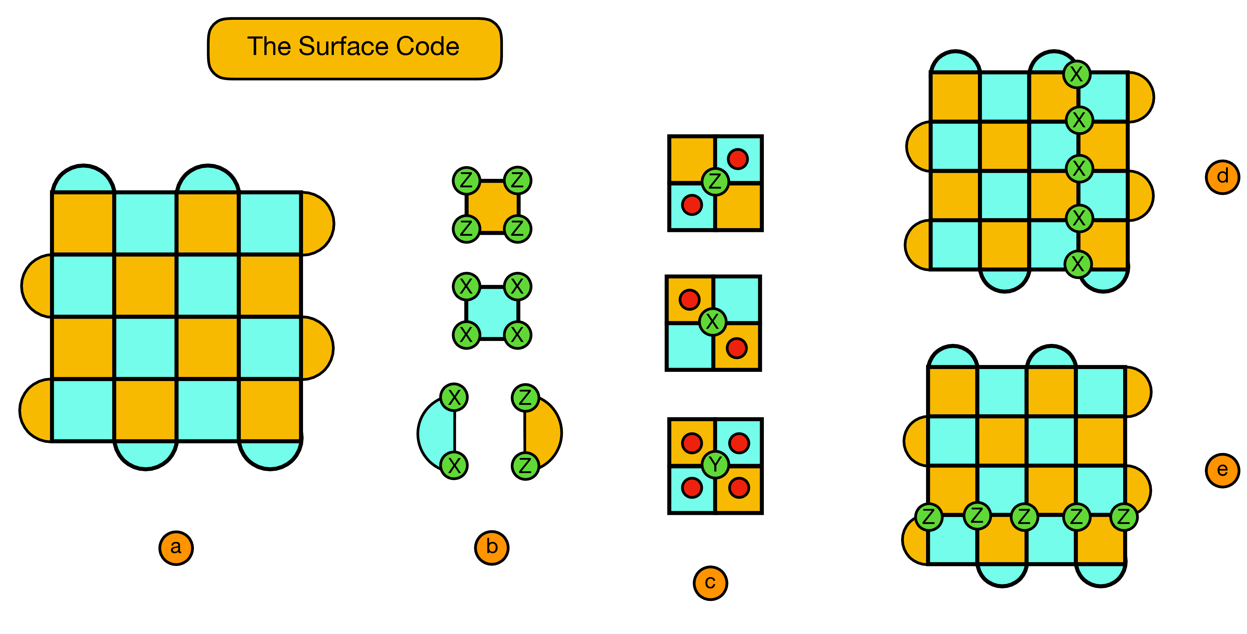
• We consider a d by d lattice, with qubits on the vertices (referred to as physical qubits), and plaquette stabilizers (a).
• Orange (blue) plaquettes indicate stabilizers which check the Z (X) parity of qubits on the vertices of the plaquette (b).
• Using red circles to indicate violated stabilizers we see here some basic examples of the syndromes created from X, Y or Z Pauli flips on a given vertex qubit (c).
• The X logical operator of the surface code we consider is given by any continuous string of X errors which connect the top and bottom boundaries of the code (d).
• Similarly, The Z logical operator is given by any continuous string of Z errors which connect the left and right boundaries of the code (e).

In order to get intuition for the decoding problem, which we will present in detail further down, it is useful to see some examples of the syndromes (configurations of violated stabilizers) generated by various error configurations...

In particular, it is very important to note that the map from syndromes to error configurations is not one-to-one! For example, one can see that the error configurations given in the top-left and bottom-left codes both lead to the same syndrome. This ambiguity in the error configuration leading to a given syndrome gives rise to the decoding problem, which we describe below.

1b) The Decoding Problem

Given the above introduction to the surface code it is now possible to understand the decoding problem, within the fault tolerant setting. Quite loosely, given any state in the ground state space of the code, the aim of decoding is keep the code in this given state by exploiting faulty syndrome information to determine which corrections need to be applied to the code to compensate for continuous noise and errors.

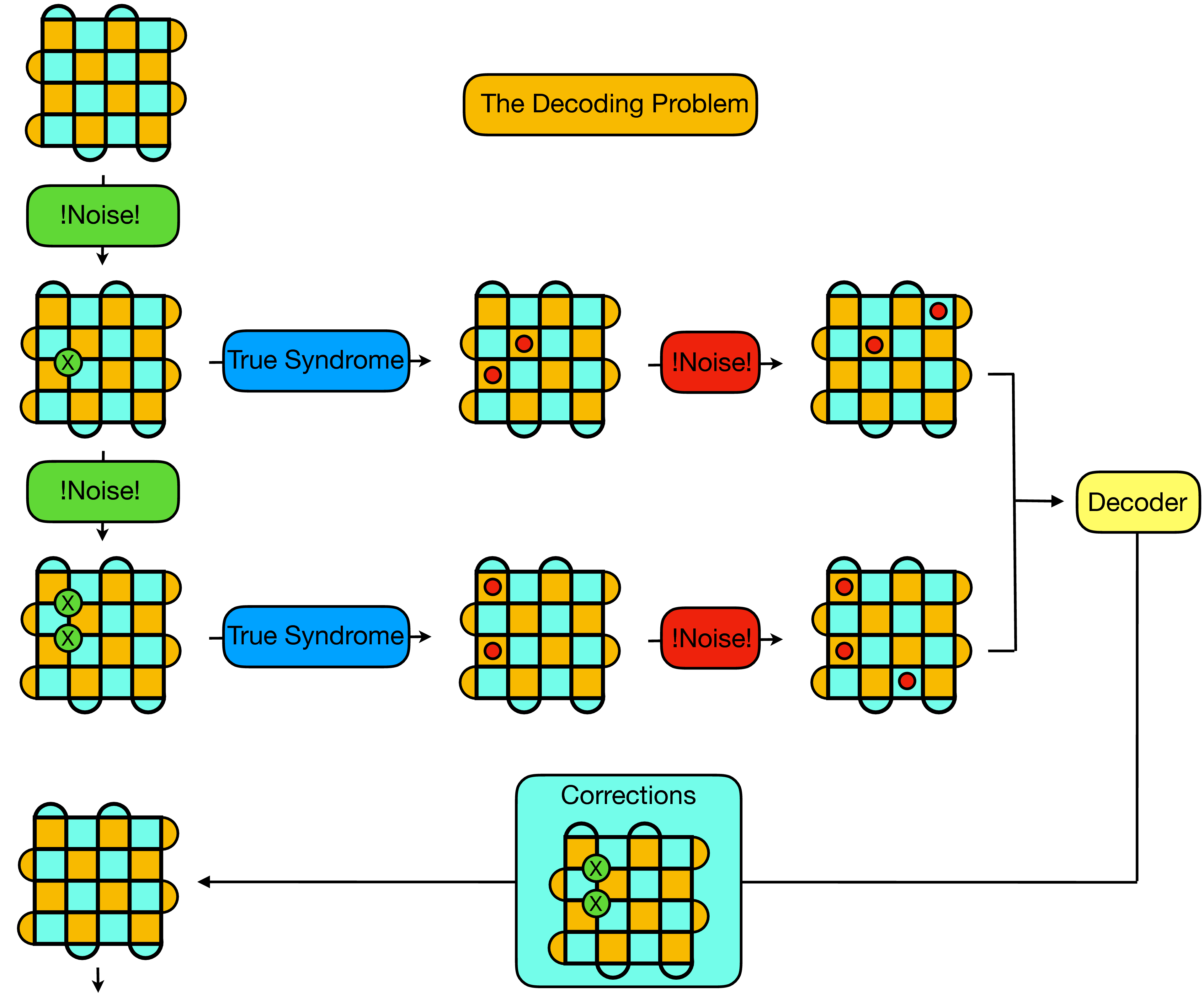
To be more specific, let's consider the above illustration:

1. In the top left, we start with a state in the code space - i.e. a state for which no stabilizers are violated. Our goal is to maintain the logical qubit in this state.
2. Now, while storing the logical qubit (between gates for instance) the physical qubits are subject to noise. We consider depolarizing noise here for simplicity, for which in each unit of time each physical qubit is subject to either a Pauli X, Y or Z flip with a given probability (the physical error rate). In the above illustration, we imagine an X flip occurring on the physical qubit in the third row and second column.
3. In order to maintain the code in the state it was given to us, we therefore need to perform a correction by applying an X gate to the qubit which was randomly flipped. To do this, we need perform a syndrome extraction, from which our decoding algorithm can attempt to diagnose the error configuration which gave rise to the received syndrome. However, as illustrated in the diagram, the syndrome extraction process is also noisy, and for each stabilizer there is a probability (the measurement error rate) that the measured stabilizer value is incorrect - i.e. that we see a violated stabilizer where there is not one, or no violated stabilizer where there actually is one.
4. To deal with this situation, instead of providing a single syndrome to the decoder, we perform multiple (faulty) syndrome measurements, between which physical errors may also occur. We then provide as input to our decoder not a single syndrome, but a stacked volume of successive syndrome slices.
5. From this syndrome volume the decoding algorithm needs to suggest corrections which when applied to the code lattice move the logical qubit back into the original state (in practice, these corrections are not actually implemented, but rather tracked through the computation, and applied in a single step at the end).
6. In the ideal case the decoder will be able to correctly diagnose a sufficient proportion of syndrome volumes, such that the probability of an error occurring on the logical qubit is lower than the physical error rate on a physical qubit.

1c) DeepQ Learning as a Tool for Obtaining Decoders

Given the problem as specified above, we utilize DeepQ reinforcement learning, a technique which has been successfully used to obtain agents capable of super-human performance in domains such as Atari, to obtain decoders which are capable of dealing with faulty measurements up to a threshold physical and measurement error rate. We will not go too deeply into the details and theory of Q-learning here, as an excellent introduction can be found in the fantastic textbook of Sutton and Barto, which is strongly recommended.

However, to give a brief overview, the rough idea is that we will utilize a deep neural network (a convolutional neural network in our case) to parameterize the Q-function of a decoding agent, which interacts with the code lattice (the environment). This Q-function is a function which maps from states of the environment - syndrome volumes plus histories of previously applied corrections - to a Q-value for each available correction, where the Q-value of a given action, with respect to a particular environment state, encodes the expected long term benefit (not the exact technical definition!) to the agent of applying that correction when in that state. Given the Q-values corresponding to a given environment state, the optimal correction strategy then corresponds to applying the correction with the largest Q-value. Within this framework, the goal is then to obtain the optimal Q-function, which is done by letting the agent interact with the environment, during which the agents experiences are used to iteratively update the Q-function.

In order to present our approach it is therefore necessary to discuss:

• The manner in which we encode the environment state.
• The parameterization of our Q-function via a deep neural network.
• The procedure via which the agent interacts with the environment to gain experience, from which the Q-function can be updated.

Let's begin with the manner in which the environment state is encoded. In particular, at any given time we consider the environment state to consist of:

1. A representation of the most recently measured faulty syndrome volume.
2. A representation of the actions which have been taken since receiving the most recent syndrome volume.

Given a d by d surface code lattice, we encode a single syndrome slice in a (2d+1) by (2d + 1) binary matrix, as illustrated below:

Similarly, we encode the history of either X or Z Pauli corrections applied since the last syndrome volume was received in a (2d+1) by (2d + 1) binary matrix of the following form:

Finally, given these conventions for syndrome and action history slices we can construct the complete environment state by stacking syndrome slices on top of an action history slice for each allowed Pauli operator (in practice we only need to allow for X and Z corrections). This gives us a total environment state in this form:

In the above image we have shown just three syndrome slices for simplicity, but as we will see later the depth of the syndrome volume (the number of slices) can be chosen at will.

Now that we know how the state of the environment is encoded at any given time step we can proceed to examine the way in which we choose to parameterize the Q-function of our agent via a deep convolutional neural network. For an introduction to such networks, see here or here.

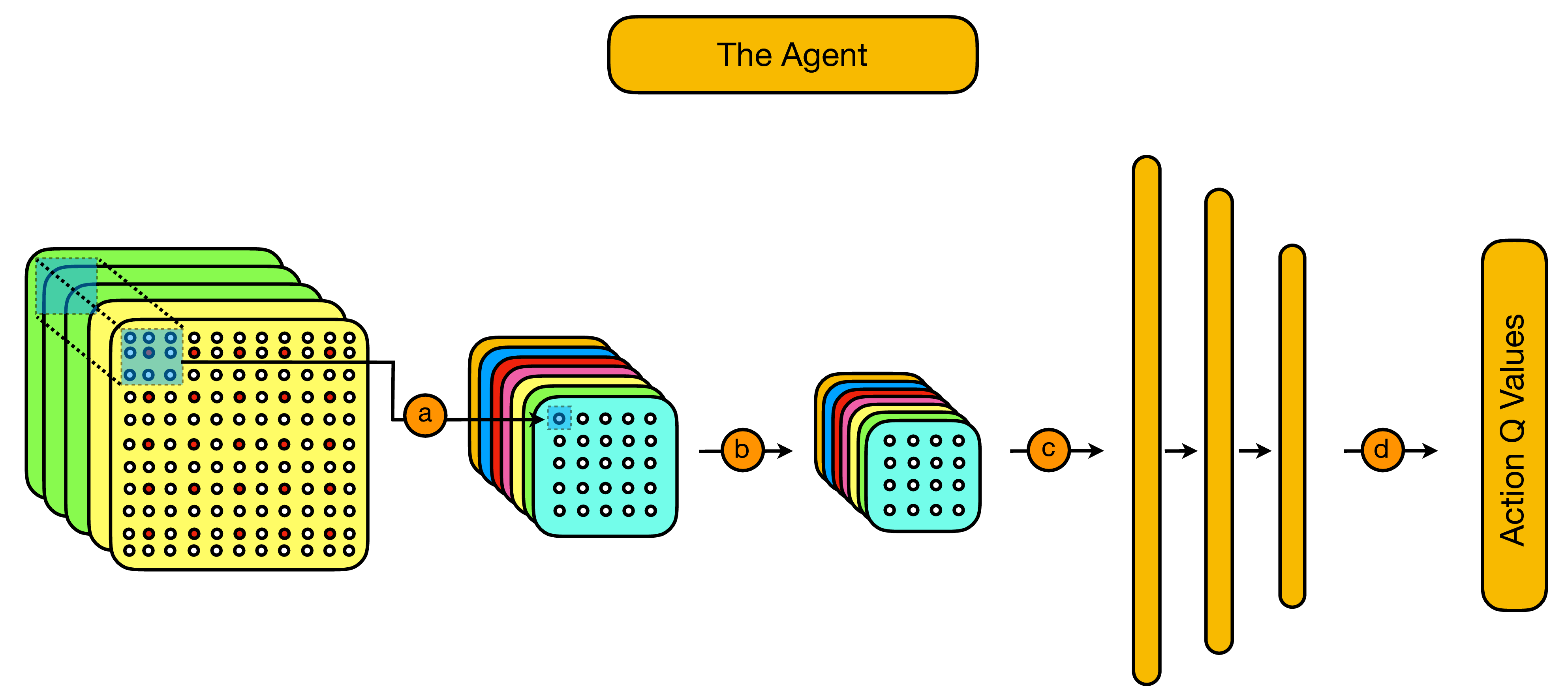
As illustrated above, our deepQ network is given by a simple convolutional neural network, consisting of:

1. A user-specified number of convolutional layers (a-b).
2. A user specified number of feed-forward layers (c).
3. A final layer providing Q-values for each available correction (d), with respect to the input state.

Given these ingredients we can now examine in detail the training procedure, through which an optimal Q-function is updated via iterative updates from experience generated by interaction with the environment. As per the majority of reinforcement learning techniques, and illustrated below, this procedure involves a sequence of alternating steps in which:

1. The environment provides a state to the agent.
2. The agent uses its current strategy to choose an action, with which it acts on the environment.
3. The environment updates its internal state appropriately, and responds to the agent by providing a new state along with a numerical reward and a binary signal which illustrates whether the agent is "dead" or "alive".
4. If the agent hasn't "died", it can then use this reward signal to update its internal strategy before once again acting on the environment and starting another round of interaction. If it has died, a new episode is started.

From the agent's perspective the goal is to converge to a strategy which allows it to maximise the expected value of its (discounted) cumulative reward. In our particular context of the decoding problem, an episode works as illustrated below:

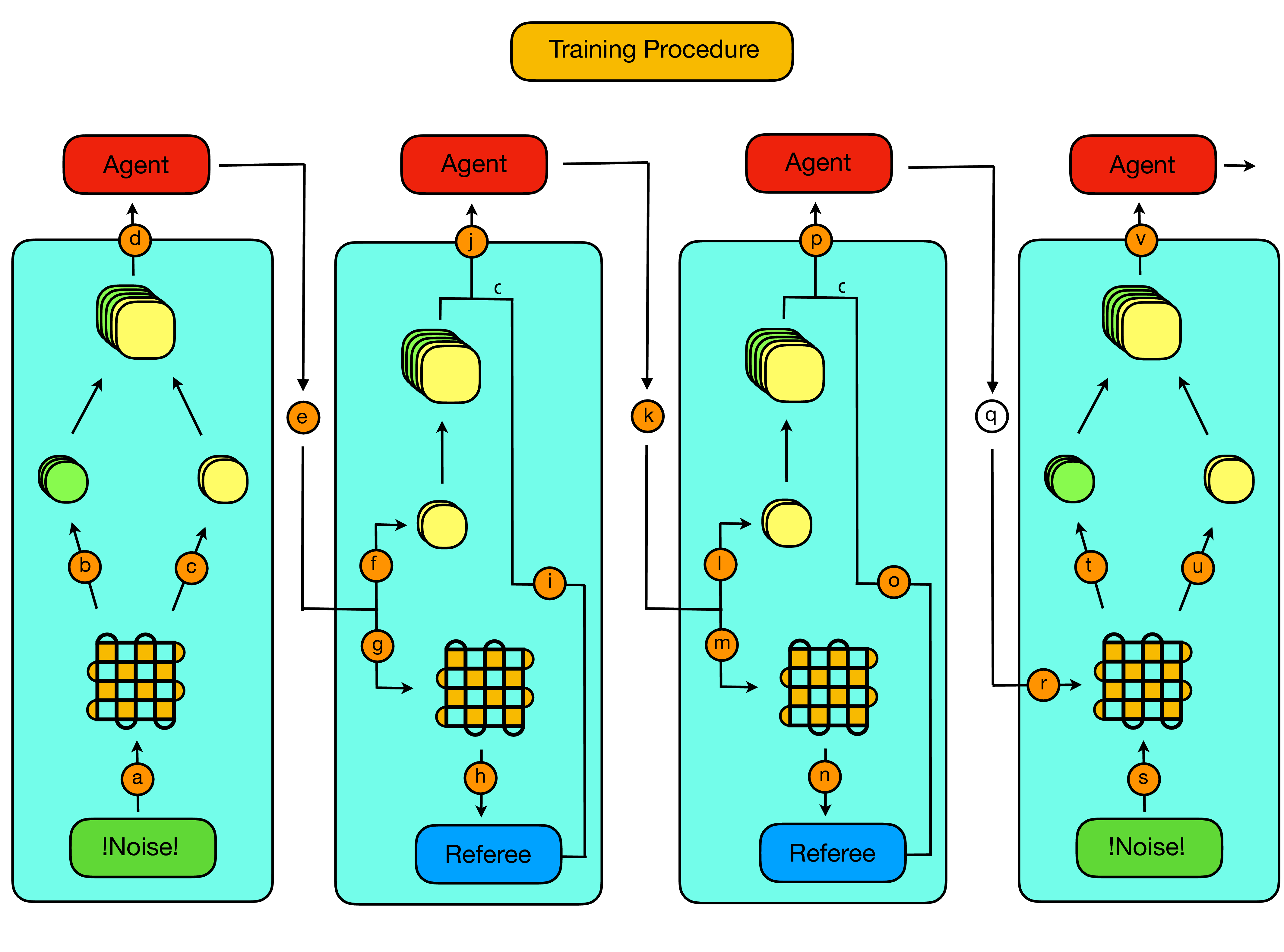
In particular:

1. As illustrated and described in Section 1b. (the "Decoding Problem"), an episode starts with the extraction of a (faulty) syndrome volume from the code (a, b). If the syndrome volume is trivial, i.e. there is not a single violated stabilizer in the entire volume, then another syndrome volume is extracted.
2. As a new syndrome volume has just been extracted, the action history is reset to all zeros (c).
3. The just extracted syndrome volume is combined with the reset action history, as previously described in the "state construction" figure, and then provided to the agent as the initial state (d).
4. Now the agent must choose an action (e). As per most RL algorithms it is helpful to balance a period of exploration, with a period of exploiting previously obtained knowledge. As such, with a given probability \epsilon, which is annealed during the course of training, the agent will choose an action at random, and with a probability 1-\epsilon the agent will choose the action with the maximal Q-value according to its current parameterization. In order to aid training, we restrict the agents random choice to actions which are either adjacent to violated stabilizer, or adjacent to previously acted on qubits.
5. When the agents acts on the environment with the chosen action, provided the action is not the identity action (request new syndrome action), multiple things then happen simultaneously. Firstly, the action history slices of the visible state are updated to indicate the action that has been applied (f). Then, the action is actually applied to the code lattice, whose error configuration is updated accordingly (g). Then finally, in order to determine the reward, a "referee" decoder takes in the true non-faulty syndrome corresponding to the updated error configuration (h). If the referee decoder can succesfully decode the current syndrome, then the agent remains alive and the episode continues, if not then the agent dies and the episode ends. If the agent remains alive and its action has resulted in putting the code back into the desired initial state, the agent is giving a reward of 1, in any other case the agent is given a reward of 0.
6. The reward and game over signal is then combined with the updated state (in which only the action history was updated) and provided to the agent (i,j). In addition, the tuple of (state, action, reward, new state, game_over) is added to an external memory which is used to update the parametrization of the agent via backpropagation.
7. The procedure detailed above is then repeated (k-p) until the point at which the agent chooses to do the identity (q), which can be done explicitly, or by repeating an action. Conceptually, the identity action is meant as a tool for the agent to signal its belief that it has applied all the corrections necessary to return the code to the desired initial state.
8. Given the identity signal from the agent, the environment then provides a new faulty syndrome volume (s,t), the action history slices of the state are reset, the new visible state is constructed from the rest action history and the updated syndrome (u,t) and fed to the agent, from which the episode continues as per steps (4-7), until the agent dies.

What has not been specifically illustrated in the above diagram is the procedure via which the parametrization of the Q-function is updated from batches of experience tuples. We will not present the details here as this is done using the exact same Q learning methodology described in these two landmark papers on deepQ learning.

At this point all that remains is to discuss how decoding is done in practice once training has been completed and the agent has converged to an optimal Q-function. As illustrated below, this is quite straightforward:

Specifically, decoding proceeds as follows:

1. Firstly, a syndrome volume is extracted from the code lattice and encoded as previously discussed (a,b). This encoded syndrome volume is then stacked with a blank action history to create the initial input state to the decoder (c, d).
2. Given this input state, one forward pass of the neural network is executed and an argmax is taken over the output Q-values to obtain the first suggested correction. This suggested correction is then added to a memory (f) and used to update the action history slices of the visible state (e). These updated action history slices are then combined with the original syndrome volume (g) and passed to the decoder (h)
3. Step 2 is then repeated (i,j,k,l) until the point at which the agent chooses the identity action (m).
4. At this point, given that the agent has signalled that it believes it has supplied all the necessary corrections, the accumulated corrections are applied to the code lattice (n), or in practice, tracked through the computation.

2) Training Decoders in Practice

Now that we have discussed the conceptual foundations, strategies and techniques involved, we will provide detailed examples of how train decoders via the procedures discussed. In particular, we will first walk through a very simple script for training a decoder with a given set of hyper-parameters, which will lay the foundation for the discussion in Section 4 of how to perform a large scale iterated training procedure, involving multiple hyper-parameter optimizations at each stage, in order to obtain optimal decoders over a large range of error rates.

If you would like to run the code discussed in this section, you can find the simple single point training script within the "Training Example" notebook in the example_notebooks folder of the repo.

2a) Requirements

The following packages are required, and can be installed via PIP:

1. Python 3 (with numpy and scipy)
2. tensorflow
3. keras
4. gym

In addition, a modified version of the Keras-RL package is required, which should be installed from this fork

2b) A Simple Training Script

We begin by importing all required packages and methods:

import numpy as np
import keras
import tensorflow
import gym

from Function_Library import *
from Environments import *

import rl as rl
from rl.agents.dqn import DQNAgent
from rl.policy import BoltzmannQPolicy, EpsGreedyQPolicy, LinearAnnealedPolicy, GreedyQPolicy
from rl.memory import SequentialMemory
from rl.callbacks import FileLogger

import json
import copy
import sys
import os
import shutil
import datetime

We then proceed by providing all required hyperparameters and physical configuration settings. In order to allow for easier grid searching and incremented training later on we choose to split all hyperparameters into two categories:

• fixed configs: These remain constant during the course of a grid search or incremented training procedure.
• variable configs: We will later set up training grids over these hyperparameters.

In particular, the fixed parameters one must provide are:

1. d: The lattice width (equal to the lattice height)
2. use_Y: If true then the agent can perform Y Pauli flips directly, if False then the agent can only perform X and Z Pauli flips.
3. train_freq: The number of agent-environment interaction steps which occur between each updating of the agent's weights.
4. batch_size: The size of batches used for calculating loss functions for gradient descent updates of agent weights.
5. print_freq: Every print_freq episodes the statistics of the training procedure will be logged.
6. rolling_average_length: The number of most recent episodes over which any relevant rolling average will be calculated.
7. stopping_patience: The number of episodes after which no improvement will result in the early stopping of the training procedure.
8. error_model: A string in ["X", "DP"], specifiying the noise model of the environment as X flips only or depolarizing noise.
9. c_layers: A list of lists specifying the structure of the convolutional layers of the agent deepQ network. Each inner list describes a layer and has the form [num_filters, filter_width, stride].
10. ff_layers: A list of lists specifying the structure of the feed-forward neural network sitting on top of the convolutional neural network. Each inner list has the form [num_neurons, output_dropout_rate].
11. max_timesteps: The maximum number of training timesteps allowed.
12. volume_depth: The number of syndrome measurements taken each time a new syndrome extraction is performed - i.e. the depth of the syndrome volume passed to the agent.
13. testing_length: The number of episodes uses to evaluate the trained agents performance.
14. buffer_size: The maximum number of experience tuples held in the memory from which the update batches for agent updating are drawn.
15. dueling: A boolean indicating whether or not a dueling architecture should be used.
16. masked_greedy: A boolean which indicates whether the agent will only be allowed to choose legal actions (actions next to a violated stabilizer or previously flipped qubit) when acting greedily (i.e. when choosing actions via the argmax of the Q-values)
17. static_decoder: For training within the fault tolerant setting (multi-cycle decoding) this should always be set to True.

In addition, the parameters which we will later incrementally vary or grid search around are:

1. p_phys: The physical error probability
2. p_meas: The measurement error probability
3. success_threshold: The qubit lifetime rolling average at which training has been deemed succesfull and will be stopped.
4. learning_starts: The number of initial steps taken to contribute experience tuples to memory before any weight updates are made.
5. learning_rate: The learning rate for gradient descent optimization (via the Adam optimizer)
6. exploration_fraction: The number of time steps over which epsilon, the parameter controlling the probability of a random explorative action, is annealed.
7. max_eps: The initial maximum value of epsilon.
8. target_network_update_freq: In order to achieve stable training, a target network is cloned off from the active deepQ agent every target_network_update_freq interval of steps. This target network is then used to generate the target Q-function over the following interval.
9. gamma: The discount rate used for calculating the expected discounted cumulative return (the Q-values).
10. final_eps: The final value at which annealing of epsilon will be stopped.

Furthermore, in addition to all the above parameters one must provide a directory into which results and training progress as logged, as well as the path to a pre-trained referee decoder. Here e provide two pre-trained feed forward classification based referee decoders, one for X noise and one for DP noise. However, in principle any perfect-measurement decoding algorithm (such as MWPM) could be used here.

fixed_configs = {"d": 5,
                "use_Y": False,
                "train_freq": 1,
                "batch_size": 32,
                "print_freq": 250,
                "rolling_average_length": 500,
                "stopping_patience": 500,
                "error_model": "X",
                "c_layers": [[64,3,2],[32,2,1],[32,2,1]],
                "ff_layers": [[512,0.2]],
                "max_timesteps": 1000000,
                "volume_depth": 5,
                "testing_length": 101,
                "buffer_size": 50000,
                "dueling": True,
                "masked_greedy": False,
                "static_decoder": True}

variable_configs = {"p_phys": 0.001,
                    "p_meas": 0.001,
                    "success_threshold": 10000,
                    "learning_starts": 1000,
                    "learning_rate": 0.00001,
                    "exploration_fraction": 100000,
                    "max_eps": 1.0,
                    "target_network_update_freq": 5000,
                    "gamma": 0.99,
                    "final_eps": 0.02}

logging_directory = os.path.join(os.getcwd(),"logging_directory/")
static_decoder_path = os.path.join(os.getcwd(),"referee_decoders/nn_d5_X_p5")


all_configs = {}

for key in fixed_configs.keys():
    all_configs[key] = fixed_configs[key]

for key in variable_configs.keys():
    all_configs[key] = variable_configs[key]

static_decoder = load_model(static_decoder_path)                                                 
logging_path = os.path.join(logging_directory,"training_history.json")
logging_callback = FileLogger(filepath = logging_path,interval = all_configs["print_freq"])

Now that we have specified all the required parameters we can instantiate our environment:

env = Surface_Code_Environment_Multi_Decoding_Cycles(d=all_configs["d"], 
    p_phys=all_configs["p_phys"], 
    p_meas=all_configs["p_meas"],  
    error_model=all_configs["error_model"], 
    use_Y=all_configs["use_Y"], 
    volume_depth=all_configs["volume_depth"],
    static_decoder=static_decoder)

The environment class is defined to mirror the environments of [https://gym.openai.com/](openAI gym), and such contains the required "reset" and "step" methods, via which the agent can interact with the environment, in addition to decoding specific methods and attributes whose details can be found in the relevant method docstrings.

We can now proceed to define the agent. We being by specifying the memory to be used, as well as the exploration and testing policies.

memory = SequentialMemory(limit=all_configs["buffer_size"], window_length=1)

policy = LinearAnnealedPolicy(EpsGreedyQPolicy(masked_greedy=all_configs["masked_greedy"]), 
    attr='eps', value_max=all_configs["max_eps"], 
    value_min=all_configs["final_eps"], 
    value_test=0.0, 
    nb_steps=all_configs["exploration_fraction"])

test_policy = GreedyQPolicy(masked_greedy=True)

Finally, we can then build the deep convolutional neural network which will represent our Q-function and compile our agent.

model = build_convolutional_nn(all_configs["c_layers"], 
                               all_configs["ff_layers"], 
                               env.observation_space.shape, 
                               env.num_actions)

dqn = DQNAgent(model=model, 
               nb_actions=env.num_actions, 
               memory=memory, 
               nb_steps_warmup=all_configs["learning_starts"], 
               target_model_update=all_configs["target_network_update_freq"], 
               policy=policy,
               test_policy = test_policy,
               gamma = all_configs["gamma"],
               enable_dueling_network=all_configs["dueling"])  


dqn.compile(Adam(lr=all_configs["learning_rate"]))

With both the agent and the environment specified, it is then possible to train the agent by calling the agent's "fit" method. If you want to run this on a single computer, be careful, it may take up to 12 hours!

now = datetime.datetime.now()
started_file = os.path.join(logging_directory,"started_at.p")
pickle.dump(now, open(started_file, "wb" ) )

history = dqn.fit(env, 
  nb_steps=all_configs["max_timesteps"], 
  action_repetition=1, 
  callbacks=[logging_callback], 
  verbose=2,
  visualize=False, 
  nb_max_start_steps=0, 
  start_step_policy=None, 
  log_interval=all_configs["print_freq"],
  nb_max_episode_steps=None, 
  episode_averaging_length=all_configs["rolling_average_length"], 
  success_threshold=all_configs["success_threshold"],
  stopping_patience=all_configs["stopping_patience"],
  min_nb_steps=all_configs["exploration_fraction"],
  single_cycle=False)

During the training procedure various statistics are logged, at the specified episode frequency, to both stdout and to the file "training_history.json" in the specified directory:

Training for 1000000 steps ...
-----------------
                
Episode: 250
Step: 2232/1000000
This Episode Steps: 4
This Episode Reward: 0.0
This Episode Duration: 0.122s
Rolling Lifetime length: 38.000
Best Lifetime Rolling Avg: 52.857142857142854
Best Episode: 6
Time Since Best: 243
Has Succeeded: False
Stopped Improving: False
Metrics: loss: 0.024631, mean_q: 0.104172, mean_eps: 0.978151
Total Training Time: 42.201s

-----------------
                
Episode: 500
Step: 4482/1000000
This Episode Steps: 7
This Episode Reward: 1.0
This Episode Duration: 0.201s
Rolling Lifetime length: 39.290
Best Lifetime Rolling Avg: 52.857142857142854
Best Episode: 6
Time Since Best: 493
Has Succeeded: False
Stopped Improving: False
Metrics: loss: 0.023562, mean_q: 0.120933, mean_eps: 0.956116
Total Training Time: 106.792s

And training goes on...

-----------------
                
Episode: 6000
Step: 89611/1000000
This Episode Steps: 37
This Episode Reward: 24.0
This Episode Duration: 1.061s
Rolling Lifetime length: 279.420
Best Lifetime Rolling Avg: 279.42
Best Episode: 5999
Time Since Best: 0
Has Succeeded: False
Stopped Improving: False
Metrics: loss: 0.343747, mean_q: 4.159633, mean_eps: 0.121998
Total Training Time: 2478.817s

-----------------
                
Episode: 6250
Step: 126262/1000000
This Episode Steps: 784
This Episode Reward: 566.0
This Episode Duration: 21.441s
Rolling Lifetime length: 1020.830
Best Lifetime Rolling Avg: 1020.83
Best Episode: 6249
Time Since Best: 0
Has Succeeded: False
Stopped Improving: False
Metrics: loss: 0.580168, mean_q: 9.287714, mean_eps: 0.020000
Total Training Time: 3490.853s

Training Finished in 5840.354 seconds
        
Final Step: 210321
Succeeded: False
Stopped_Improving: False
Final Episode Lifetimes Rolling Avg: 2882.750

As you can see above, we manually stopped training after approximately 6000 seconds while the agent was still improving, and before it has reached the specified success threshold.

In order to evaluate the agent later on, or apply the agent in a production decoding scenario we can easily save the weights:

weights_file = os.path.join(logging_directory, "dqn_weights.h5f")
dqn.save_weights(weights_file, overwrite=True)

And finally, in order to evaluate the training procedure we may be interested in viewing any of the metrics which were logged. These are all saved within the history.history dictionary. For example, we are often most interested in analyzing the training procedure by looking at the rolling average of the qubit lifetime, which we can do as follows:

from matplotlib import pyplot as plt
%matplotlib inline

training_history = history.history["episode_lifetimes_rolling_avg"]

plt.figure(figsize=(12,7))
plt.plot(training_history)
plt.xlabel('Episode')
plt.ylabel('Rolling Average Qubit Lifetime')
_ = plt.title("Training History")

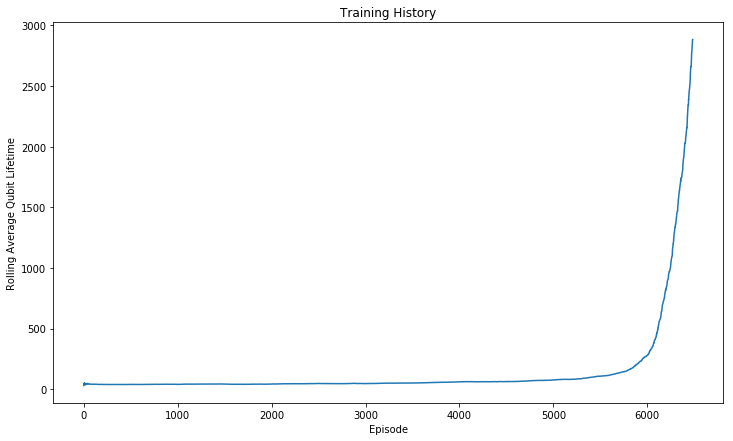
From the above plot one can see that during the exploration phase the agent was unable to do well, due to constant exploratory random actions, but was able to exploit this knowledge effectively once the exploration probability became sufficiently low. Again, it is also clear that the agent was definitely still learning and improving when we chose to stop the training procedure.

3) Evaluating and Running Decoders

Now that we know how to train a decoder, we would like to see how to evaluate the performance of that decoder, as well as how to use the decoder in a production setting. In this section we will demonstrate how to perform both of these tasks. Once again, all of this code can be found within the "Testing Examples" notebook of the example_notebooks folder of the repo.

3a) Evaluating a Trained Decoder

Given a trained decoder we would of course like to benchmark the decoder to evaluate how well it performs. This procedure is very similar to training the decoder, in that we run multiple decoding episodes in which the agent interacts with the environment until it "dies" - however in this context we would like the agent to use only a greedy policy for action selection, i.e. to never make random moves, and we do not need to update the agents parameters in time. As we will see benchmarking an agent is made easy by use of the DQNAgent class "test" method.

Again, we begin by importing the necessary packages:

import numpy as np
import keras
import tensorflow
import gym

from Function_Library import *
from Environments import *

import rl as rl
from rl.agents.dqn import DQNAgent
from rl.policy import BoltzmannQPolicy, EpsGreedyQPolicy, LinearAnnealedPolicy, GreedyQPolicy
from rl.memory import SequentialMemory
from rl.callbacks import FileLogger

import json
import copy
import sys
import os
import shutil
import datetime

Using TensorFlow backend.

Now, we need to load:

1. The hyper-parameters of the agent we would like to test
2. The weights of the agent

In this example we will evaluate one of the provided pre-trained decoders, for d=5, with X noise only, trained at an error rate of p_phys=p_meas=0.007

fixed_configs_path = os.path.join(os.getcwd(),"../trained_models/d5_x/fixed_config.p")
variable_configs_path = os.path.join(os.getcwd(),"../trained_models/d5_x/0.007/variable_config_77.p")
model_weights_path = os.path.join(os.getcwd(),"../trained_models/d5_x/0.007/final_dqn_weights.h5f")

static_decoder_path = os.path.join(os.getcwd(),"referee_decoders/nn_d5_X_p5")
static_decoder = load_model(static_decoder_path)

fixed_configs = pickle.load( open(fixed_configs_path, "rb" ) )
variable_configs = pickle.load( open(variable_configs_path, "rb" ) )

all_configs = {}

for key in fixed_configs.keys():
    all_configs[key] = fixed_configs[key]

for key in variable_configs.keys():
    all_configs[key] = variable_configs[key]

Now we can instantiate the environment in which we will test the agent:

env = Surface_Code_Environment_Multi_Decoding_Cycles(d=all_configs["d"], 
    p_phys=all_configs["p_phys"], 
    p_meas=all_configs["p_meas"],  
    error_model=all_configs["error_model"], 
    use_Y=all_configs["use_Y"], 
    volume_depth=all_configs["volume_depth"],
    static_decoder=static_decoder)

Now we build a model and instantiate an agent with all the parameters of the pre-trained agent. Notice that we insist on a greedy policy!

model = build_convolutional_nn(all_configs["c_layers"],all_configs["ff_layers"], 
                               env.observation_space.shape, env.num_actions)
memory = SequentialMemory(limit=all_configs["buffer_size"], window_length=1)
policy = GreedyQPolicy(masked_greedy=True)
test_policy = GreedyQPolicy(masked_greedy=True)

# ------------------------------------------------------------------------------------------

dqn = DQNAgent(model=model, 
               nb_actions=env.num_actions, 
               memory=memory, 
               nb_steps_warmup=all_configs["learning_starts"], 
               target_model_update=all_configs["target_network_update_freq"], 
               policy=policy,
               test_policy=test_policy,
               gamma = all_configs["gamma"],
               enable_dueling_network=all_configs["dueling"])  


dqn.compile(Adam(lr=all_configs["learning_rate"]))

At this stage the agent has random weights, and so we load in the weights of the pre-trained agent:

dqn.model.load_weights(model_weights_path)

And now finally we can benchmark the agent using the test method.

It is important to note that the reported episode length is the number of non-trivial syndrome volumes that the agent received, as these are the steps during which a decision needs to be taken on the part of the agent. The qubit lifetime, whose rolling average is reported, is the total number of syndrome measurements (between which an error may occur) for which the agent survived, as this is the relevant metric to compare with a single faulty qubit whose expected lifetime is 1/(error_probability).

nb_test_episodes = 1001
testing_history = dqn.test(env,nb_episodes = nb_test_episodes, visualize=False, verbose=2, 
                           interval=100, single_cycle=False)

Testing for 1001 episodes ...
-----------------
Episode: 1
This Episode Length: 44
This Episode Reward: 27.0
This Episode Lifetime: 125

Episode Lifetimes Avg: 125.000

-----------------
Episode: 101
This Episode Length: 278
This Episode Reward: 171.0
This Episode Lifetime: 830

Episode Lifetimes Avg: 330.149

and the evaluation continues...

-----------------
Episode: 901
This Episode Length: 230
This Episode Reward: 172.0
This Episode Lifetime: 685

Episode Lifetimes Avg: 330.638

-----------------
Episode: 1001
This Episode Length: 280
This Episode Reward: 166.0
This Episode Lifetime: 765

Episode Lifetimes Avg: 329.106

results = testing_history.history["episode_lifetime"]

print("Mean Qubit Lifetime:", np.mean(results))

Mean Qubit Lifetime: 329.1058941058941

Here we see that on average, over 1001 test episodes, the qubit survives for 329 syndrome measurements on average, which is better than the average lifetime of 143 syndrome measurements for a single faulty qubit.

3b) Using a Trained Decoder in Production

In addition to benchmarking a decoder via the agent test method, we would like to demonstrate how to use the decoder in practice, given a faulty syndrome volume. In principle all the information on how to do this is contained within the environments and test method, but to aid in applying these decoders quickly and easily in practice we make everything explicit here:

To do this, we start by generating a faulty syndrome volume as would be generated by an experiment or in the process of a quantum computation:

d=5
p_phys=0.007
p_meas=p_phys
error_model = "X"
qubits = generateSurfaceCodeLattice(d)

hidden_state = np.zeros((d, d), int)

faulty_syndromes = []
for j in range(d):
    error = generate_error(d, p_phys, error_model)
    hidden_state = obtain_new_error_configuration(hidden_state, error)
    current_true_syndrome = generate_surface_code_syndrome_NoFT_efficient(hidden_state, qubits)
    current_faulty_syndrome = generate_faulty_syndrome(current_true_syndrome, p_meas)
    faulty_syndromes.append(current_faulty_syndrome)

By viewing the final hidden_state (the lattice state) we can see what errors occured, which here was a single error on the 21st qubit (we start counting from 0, and move row wise left to right).

print(hidden_state)

[[0. 0. 0. 0. 0.]
 [0. 0. 0. 0. 0.]
 [0. 0. 0. 0. 0.]
 [0. 0. 0. 0. 0.]
 [0. 1. 0. 0. 0.]]

And we can view the faulty_syndromes that we received, which is what would come out of an experiment. As we can see, measurement errors occurred in syndrome slices 2 and 5, and it appears as if the actual error occurred between extraction of syndrome 2 and 3:

for j in range(d):
    print("syndrome slice", j+1)
    print()
    print(faulty_syndromes[j])
    print()

syndrome slice 1

[[0 0 0 0 0 0]
 [0 0 0 0 0 0]
 [0 0 0 0 0 0]
 [0 0 0 0 0 0]
 [0 0 0 0 0 0]
 [0 0 0 0 0 0]]

syndrome slice 2

[[0 0 0 0 0 0]
 [0 0 1 0 0 0]
 [0 0 0 0 1 0]
 [0 0 0 0 0 0]
 [0 0 0 0 0 0]
 [0 0 0 0 0 0]]

syndrome slice 3

[[0 0 0 0 0 0]
 [0 0 0 0 0 0]
 [0 0 0 0 0 0]
 [0 0 0 0 0 0]
 [0 1 0 0 0 0]
 [0 0 1 0 0 0]]

syndrome slice 4

[[0 0 0 0 0 0]
 [0 0 0 0 0 0]
 [0 0 0 0 0 0]
 [0 0 0 0 0 0]
 [0 1 0 0 0 0]
 [0 0 1 0 0 0]]

syndrome slice 5

[[0 1 0 0 0 0]
 [0 0 0 0 0 0]
 [0 0 0 0 0 0]
 [0 0 0 0 0 0]
 [0 1 0 0 0 0]
 [0 0 1 0 0 0]]

And now we would like to decode and obtain the suggested corrections. To do this, we begin by padding the faulty syndromes as required and by concatenating the obtained volume with an action history slice, in which all the actions are initially zero:

# Intialize a zero'd input volume
input_state = np.zeros((d+1, 2*d + 1, 2*d + 1),int)

# embed and place the faulty syndrome slices in the correct place
for j in range(d):
            input_state[j, :, :] = env.padding_syndrome(faulty_syndromes[j])

And now we can run the agent, collecting the suggested actions, until the agent does the identity, which suggests that it is finished decoding:

corrections = []

still_decoding = True
while still_decoding:
    
    # Fetch the suggested correction
    action = dqn.forward(input_state)
    
    if action not in corrections and action != env.identity_index:
        # If the action has not yet been done, or is not the identity
        
        # append the suggested correction to the list of corrections
        corrections.append(action)
        
        # Update the input state to the agent to indicate the correction it would have made
        input_state[d, :, :] = env.padding_actions(corrections)
        
    else:
        # decoding should stop
        still_decoding = False
        

And now we can view the suggested corrections, which in this case was a single correct suggestion:

print(corrections)

[21]

Note that in general if there is more than one error, or if the agent is uncertain about a given configuration, it may choose to do the identity, therefore triggering a new syndrome volume from which it may be more certain which action to take - The crucial point is that in practice we are interested in how long the qubit survives for, and an optimal strategy for achieving long qubit lifetimes may not be to attempt to fully decode into the ground state after each syndrome volume - in fact, that is one of the primary advantages of this approach!

4) Large Scale Iterative Training and Hyper-Parameter Optimization

Now that we have seen how to train and test decoders at a fixed error rate, for a given set of hyper-parameters, we would like to turn our attention to how we might be able to obtain good decoders for a large range of error rates. In order to achieve this we have developed an iterative training procedure involving hyper-parameter searches at each level of the iteration. In this section we will first outline the procedure before proceeding to discuss in detail how one can implement this procedure on a high-performance computing cluster. The scripts required for this implementation are contained in the cluster_scripts folder of the repo.

4a) Outline of the Procedure

As illustrated in the figure below, the fundemental idea is to iterate through increasing error rates, performing hyper-parameter optimizations at each iteration, and using various attributes of the optimization at one step of the iteration as a starting point for the subsequent step.

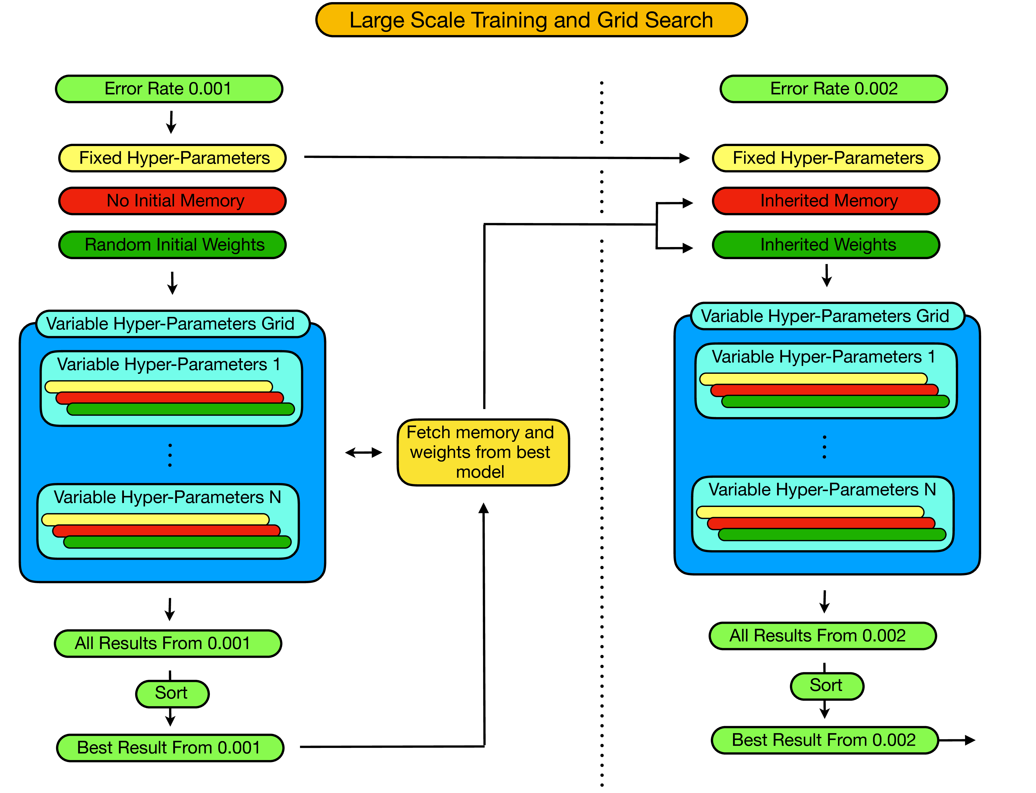
In particular, the procedure works as follows:

1. We begin by fixing the error rate to some small initial value which we estimate to be far below the threshold of the decoder and at which the agent will be able to learn a good strategy.
2. We then set the fixed hyper-parameters (as discussed in the previous section) which will remain constant throughout the entire training procedure, even as we increment the error rate.
3. Next, we create a hyper-parameter grid over the hyperparameters which we would like to optimize (the variable hyper-parameters) and proceed to train a decoder for each set of hyper-parameters in the grid. For each of these initial simulations the decoder/agent is initialized with no memory and with random initial weights.
4. For each point in the hyperparameter grid we store
   • The hyper-parameter settings for this point.
   • The entire training history.
   • The weights of the final agent.
   • The memory of the agent.
5. Additionally, for each trained agent we then evaluate the agent in "test-mode" and record the results (i.e. the average qubit lifetime one can expect when using this decoder in practice).
6. Now, given all "test-mode" results for all obtained decoders at this error rate, we then filter the results and identify the best performing decoder.
7. At this point, provided the results from just completed iteration are above some specified performance threshold, we then increase the error rate. To do this we start by fetching the experience memory and weights of the optimal decoder from the just completed iteration. Then, at the increased error rate we create a new hyper-parameter grid over the variable hyper-parameters, and train a decoder at each point in this new hyper-parameter grid. However, in this subsequent step of the iteration the agents are not initialized with random memories and weights, but with the memory and weights of the optimal performing decoder from the previous iteration.
8. This procedure then iterates until the point at which, with respect to the current error rate, the logical qubit lifetime when corrected by the optimal decoder falls beneath that of a single faulty-qubit - i.e until we are able to identify the pseudo-threshold of the decoder.

4a) Practically Implementing Large Scale Iterative Training on an HPC Cluster

In the cluster_scripts folder of the repo we provide scripts for practically implementing the above iterating training procedure on an HPC cluster using the slurm workload manager. In this section we provide detailed documentation for how to set up and implement this procedure using the provided scripts.

As an example, we will work through the iterative training procedure in detail for d=5 and X noise only, although the steps here can be easily modified to different physical scenarios, and we have also provided all the scripts necessary for d=5 with depolarizing noise.

Before beginning make sure that base "../d5_x/" directory contains:

• Environments.py
• Function_Library.py
• Controller.py
• make_executable.sh
• static_decoder (an appropriate referee decoder with the corresponding lattice size and error model)
• An empty folder called "results"
• An empty text document called "history.txt"
• A subdirectory for each error rate one would like to iterate through
• A text file "current_error_rate.txt" containing one line with the lowest error rate - i.e. 0.001

Furthermore, the subdirectory corresponding to the lowest error rate (0.001 here) should contain:

• Environments.py
• Function_Library.py
• Generate_Base_Configs_and_Simulation_Scripts.py
• Single_Point_Training_Script.py
• Start_Simulations.sh
• An empty folder "output_files"

Additionally every other error rate subdirectory should contain:

• Environments.py
• Function_Library.py
• Single_Point_Continue_Training_Script.py
• Start_Continuing_Simulations.sh
• An empty folder "output_files"

In order to run a customized/modified version of this procedure this exact directory and file structure should be replicated, as we will see below all that is necessary is to modify:

• Controller.py
• Generate_Base_Configs_and_Simulation_Scripts.py
• Providing the appropriate static/referee decoder
• Renaming the error rate subdirectories appropriately

To begin, copy the entire folder "d5_x" onto the HPC cluster and navigate into the "../d5_x/" directory. Then:

1. From "../d5_x/" start a "screen" - this provides a persistent terminal which we can later detach and re-attach at will to keep track of the training procedure, without having to remain logged in to the cluster.

   • type "screen"
   • then press enter
   • We are now in a screen

2. Run the command "bash make_executable.sh". This will allow the controller - a python script which will be run periodically to control the training process - to submit jobs via slurm.

3. Using vim or some other in-terminal editor, modify the following in Controller.py:

   • Set all the error rates that you would like to iterate through - make sure there is an appropriate subdirectory for each error rate given here. -For each error rate, provide the expected lifetime of a single faulty qubit (i.e. the threshold for decoding sucess) as well as the average qubit lifetime you would like to use as a threshold for stopping training. We recommend setting this training threshold extremely high, so that training ends due to convergence.
   • set the hyper-parameter grid that you would like to use at each error rate iteration.
   • Also make sure that all the cluster parameters (job time, nodes etc) are set correctly.
   • make sure the time threshold for evaluating whether simulations have timed out corresponds to the cluster configurations

4. Make sure history.txt is empty, make sure the results folder is empty, make sure that current_error_rate.txt contains one line with only the lowest error rate written in.

5. Navigate to the directory "../d5_x/0.001/", or in a modified scenario, the folder corresponding to the lowest error rate, again using Vim or some in-terminal editor:

   • Set the base configuration grid (fixed hyperparameters) in Generate_Base_Configs_and_Simulation_Scripts.py
   • Specify the variable hyper-parameter grid for this initial error rate.
   • Set the maximum run times for each job (each grid point will be submitted as a seperate job).
   • run this script with the command "python Generate_Base_Configs_and_Simulation_Scripts.py"

6. The previous step will have generated many configuration subdirectories, as well as a "fixed_configs.p" file in the "../d5_x/" directory one level up in the directory hierachy. Check that the fixed_configs.p file has been generated. In addition check that each "config_x" subdirectory within "../d5_x/0.001/" contains:

   • simulation_script.sh
   • variable_config_x.py

7. At this stage we then have to submit all the jobs (one for each grid point) for the initial error rate. We do this by running the command "bash Start_Simulations.sh" from inside "../d5_x/0.001/".

8. Now we have to get the script Controller.py to run periodically. Every time this script runs it will check for the current error rate and collect all available results from simulations from that error rate. If all the simulations at the specified error rate are finished, or if the time threshold for an error rate has passed, then it will write and sort the results, generate a new hyperparameter grid and simulation scripts for an increased error rate, copy the memory and weights of the optimal model from the old error rate into the appropriate directories, and submit a new batch of jobs for all the new grid points at the increased error rates. To get the controller to run periodically we do the following:

   • Navigate into the base directory "../d5_x/" containing Controller.py
   • run the command "watch -n interval_in_seconds python Controller.py"
   • eg: for ten minute intervals: "watch -n 600 Controller.py"

9. At this stage we are looking at the watch screen, which displays the difference in output between successive calls to Controller.py

   • We want to detach this screen so that we can safely logout of the cluster without interrupting training
   • To do this type ctrl+a, then d

10. We can now log out and the training procedure will continue safely, as directed by the Controller. We can log in and out of the cluster to see how training is proceeding whenever we want. In particular we can view the contents of:

    • history.txt: This file contains the result of every call to Controller.py - i.e. the current error rate, how many simulations are finished or in progress, and what action was taken.
    • results: The results folder contains text files which contain both all the results and the best result from each error rate.

11. When training is finished and we want to kill the controller we have to login to the cluster and run the following commands:

    • reattach the screen with "screen -r"
    • We are now looking at the watch output - kill this with ctrl+c
    • Now we need to kill the screen with ctrl+a and then k

5) Results

As we have discussed, during the course of the training procedure the results of all trained agents in "test_mode" are written out and stored, as well as the results from the best agent at each error rate. However, in order to ease computational time during training, each agent was only benchmarked for 100 episodes.

Here we present the full results and training histories for each best performing agent, as selected by the preliminary benchmarking during training. In particular, these full results were obtained by testing each best performing trained agent, at each error rate, for the number of episodes that guaranteed at least 10^6 syndromes were seen by the agent. All the trained agents from which these results were obtained, along with the fully detailed results (i.e. episode length of every single tested episode at each error rate for each agent), can be found in the "trained_models" directory of the repo. In addition to these evaluation results, we also provide the learning curves for all best performing agents.

The code for generating these plots, can be found in the "Final Results and Training Histories" Example Notebook, in the example notebooks folder.

We start by presenting the results obtained when using the best performing agent from each iterative training step, for both bitflip and depolarizing noise, as well as the results obtained when using the best performing agent for each specific error rate.

In addition, it is of interest to view the learning curves for all the agents whose performance is shown above. The following plots provide these training histories, along with the hyper-parameter settings for the agent, given as a list in the form [num_exploration_steps, initial_epsilon, final_epsilon, learning_rate, target_network_update_frequency].

First, let's have a look at the depolarising noise agents:

And finally, we can view the learning curves from the bitflip noise agents:

deepq-decoding's Issues

Images for readme

Images for readme

No license

There is no license associated with this project. In order to enable other people to use your code you should consider adding one. Here's a great overview of how to do it:

https://help.github.com/articles/adding-a-license-to-a-repository/

You might want to consider a copyleft license, such as GPL-3.0, which will force any derivative work to be open sourced as well.